Collections (tutorial)
A network collection is a set or sequence of several networks that belong together, e.g., by representing waves in a longitudinal network (i.e., a network observed at several moments in time). Network collections can be jointly analyzed and visualized (e.g., computing the same centrality index or applying the same layout algorithm on all open networks). A visone network collection that represents longitudinal data can be visualized by a dynamic layout algorithm showing the evolution of the network over time and it can be analyzed with the RSiena software for modeling the co-evolution of networks and behavior. This tutorial guides you through these application scenarios in an example-driven way. To follow the steps illustrated here, download the file Newfrat_top3.zip, linked from and described in the page Newcomb Fraternity (data), and extract (unzip) its content (consisting of the files newfrat01.graphml to newfrat15.graphml) to your hard disk. This tutorial assumes that you have basic knowledge about working with visone as it is illustrated in the other three basic tutorials.
Dealing with several networks (basics)
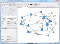
In visone, several networks can be open at the same time - each in its own network tab. In general, you can load networks into visone by (1) starting and editing a new empty network, (2) by opening a network from a local file, or (3) by creating a random network. To load the set of networks that serves as illustrating example in this tutorial, click on the menu file, open, navigate in the file browser to the directory where you've put the files newfrat01.graphml to newfrat15.graphml (see above) and select all of them before you click the ok button. (Selection of these files can be done in different ways, for instance, by keeping the Control-key pushed while successively selecting the files with a mouse left-click or by clicking on one of the files and then typing Control-a to select all files in the current directory.)
The 15 networks should be shown in 15 separate tabs in the network area. To switch between these networks, click on the name of the respective network on top of the tabs (there are little buttons with left/right-arrows on the right-hand side in the row of network names that allow you to browse through the tabs when the list of names exceeds the screen width). To close a tab, click on the X-like cross on the right-hand side of the respective tab. To close all tabs or all tabs but the current one, do a mouse right-click on one of the network names and select the appropriate option; if there are unsaved changes, visone asks you whether you want to save the files and you can answer yes/no separately for each network or chose to quit without saving any changes (click on no to all), to save all modified networks (yes to all) or chose cancel, that is not to close the tabs. (If you closed one or several of the networks, remember to open them again to follow the steps below.)
Simultaneous analysis and visualization
Network analysis and visualization algorithms can be applied to all open networks simultaneously. For instance, to compute the indegree of nodes in all 15 networks that are currently open in visone go to the analysis tab, make the appropriate choices to compute indegree (for information on this see the tutorial on visualization and analysis), and select open networks in the apply to drop-down menu at the bottom of the analysis tab before pushing the analyze! button. Each of the networks has now an attribute called indegree (or whatever name you've chosen) whose values are equal to the nodes' indegrees at the respective time points.
Applying a visualization algorithm simultaneously to all open networks works accordingly. For sake of example, map the newly computed indegree to the node size (more information about how to map attributes to graphics can be found in the tutorial on visualization and analysis).
Creating a network collection
The analysis and visualization algorithms illustrated above processed the networks separately, one at a time. So far, a node in one network has not been identified with any node in another network. To do this you have to tell visone which attribute is the one that identifies nodes by creating a network collection with the collection manager. You have to create a network collection before you compute a dynamic layout or before you model and analyze the network evolution with the RSiena interface (these two application tasks are illustrated below in this tutorial).
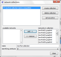
To create a network collection open the collection manager by clicking on the ![]() icon in visone's toolbar. In the collection manager push on the create collection button, select networks offered in the area labeled available networks and add them to the current collection by pushing the add button. The order in which the networks appear in the area labeled networks in collection matters since it defines the ordering of networks over time: the network in the first line corresponds to the first observation time point, that in the second line has been collected next, and so on. In our particular example, the integers 01 to 15 in the network names suggest this ordering: networks with higher numbers have been collected later. (Just for the sake of example, if network
icon in visone's toolbar. In the collection manager push on the create collection button, select networks offered in the area labeled available networks and add them to the current collection by pushing the add button. The order in which the networks appear in the area labeled networks in collection matters since it defines the ordering of networks over time: the network in the first line corresponds to the first observation time point, that in the second line has been collected next, and so on. In our particular example, the integers 01 to 15 in the network names suggest this ordering: networks with higher numbers have been collected later. (Just for the sake of example, if network newfrat12.graphml were the one collected at the last observation time you could move it to the end of the list by removing it and adding it again. It will take a few more steps to correct this and put it back on position 12.) The important option that you have to set is the identifying attribute being the name of the attribute that identifies nodes over different time points. Note that in the current example you are only offered to choose id as the identifying attribute (note that the attribute indegree is not an option for the identifying attribute since its values are not unique, i.e., several nodes have the same indegrees). While you can create a network collection even if some nodes are not present at all time points, a network collection is marked as being siena compatible if all nodes are present at all times. If a network collection is not siena compatible it cannot be modeled with RSiena but you can nevertheless compute a dynamic layout. More than one collection can be created and you can switch between them with the set as active button in the collection manager.
Dynamic visualization and animation of a network collection
Whenever there is an active network collection you can create an animation showing a movie that takes you from the first network to the last (the ordering is defined in the network collection manager). Showing such an animation in the current example will give a very bad and unstable movie - wrongly suggesting that there is enormous change from one time point to the next. The reason for this is that currently each of the networks has been layouted separately. Actually, whenever you create an animation you first have to compute a dynamic layout and scale the networks to a common bounding box before starting the animation. These points are illustrated in this section.
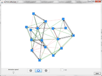
For illustration purposes, let's look at the animation without prior application of a dynamic layout. To open the animation window click on the ![]() icon in visone's toolbar. To start the animation click on the "play" button at the bottom of the animation window. The animation speed can be increased (decreased) by moving the slider to the right (left). When moving from one time point to the next, disappearing ties are colored red, new ties emerge in green color, and nodes gradually move to their new positions. Without an appropriate dynamic layout it is impossible to follow the evolution of the network structure. Indeed, while the layout at each time point shows the structure of the respective network, there is no stability at all when moving from one time point to the next.
icon in visone's toolbar. To start the animation click on the "play" button at the bottom of the animation window. The animation speed can be increased (decreased) by moving the slider to the right (left). When moving from one time point to the next, disappearing ties are colored red, new ties emerge in green color, and nodes gradually move to their new positions. Without an appropriate dynamic layout it is impossible to follow the evolution of the network structure. Indeed, while the layout at each time point shows the structure of the respective network, there is no stability at all when moving from one time point to the next.
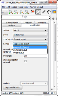
To compute a dynamic layout go to the visualization tab and chose in the drop-down menus (from top to bottom) layout, node layout, and dynamic layout. visone offers three dynamic layout methods: aggregated, anchored, and linked layout, briefly described in the following:
- aggregated layout computes the aggregation network, that is, the union of all networks in the collection. The aggregation network has as nodes all nodes that are present in at least one of the networks with links connecting nodes that are adjacent at some time point. This aggregation network is layouted once, defining the nodes' positions for all time points. The resulting animation, thus, has a maximum stability (node do not move at all) and just shows which ties emerge or disappear over time.
- anchored layout The anchored layout allows to specify a tradeoff between stability and optimal network layout at the individual time points. The nodes' positions for a single time point are computed by optimizing the quality function of stress minimization requiring at the same time that nodes are not too far from their positions in the "anchor network". (The network can be anchored at the aggregation network or at the network from the preceeding time point.) If the stability parameter is set to a high value, nodes move only slighly from one time point to the next; a low stability means that layouts at individual time points are computed paying little attention to the anchor network.
- linked layout ...
After computing a dynamic layout, click on the ![]() icon in visone's toolbar to fit all networks into a common bounding box. Then, the network collection can be animated as described above; this should now produce a much smoother animation showing the evolution of the network structure over time. Node or link properties, such as size or color, are also interpolated between animation steps - depending on what these grapical properties encode, this allows to follow the evolution of, say, centrality over time.
icon in visone's toolbar to fit all networks into a common bounding box. Then, the network collection can be animated as described above; this should now produce a much smoother animation showing the evolution of the network structure over time. Node or link properties, such as size or color, are also interpolated between animation steps - depending on what these grapical properties encode, this allows to follow the evolution of, say, centrality over time.
Statistical modeling of network dynamics
The dynamics of a network collection that is Siena compatible can be modeled via the RSiena interface. RSiena implements stochastic actor-oriented models for the evolution of networks and behavior. It allows, for instance, to test hypotheses about social influence and social selection processes in empirical longitudinal network data. The RSiena interface is started from the analysis tab by selecting task=Siena; it is required that the R connection is properly installed. More information about the RSiena interface can be found in the tutorial on using RSiena from within visone.


