Visualization and analysis (tutorial)
This tutorial shows you how analysis and visualization goes hand in hand in visone. It introduces you to the most common usage scenario: importing data from one or several files, analyzing the network, visualizing the network together with the computed indicators, exporting data and images for further processing or publication.
This tutorial assumes that you have basic knowledge about how to operate the visone GUI - as explained in the previous tutorial.
Introducing an exemplary dataset
The data that we use in this tutorial has been collected in a long-term reseach project about acculturation networks. More information about the project can be found at [1]. Among others, the personal networks of now more than 1,000 immigrants have been collected within this project. Each of the respondents (called ego) provided answers to four types of questions:
- questions about ego, including country of origin, years of residence, age, gender, skin color, reasons for migrating, health, language skills...
- alters a list of persons known to ego (for most networks the number has been fixed to 45)
- questions about alters including country of origin, country of residence, age, skin color, type of relation to ego, ...
- alter-alter ties (undirected) pairs of alters that know each other (according to the respondent)
A more detailed description is provided on the page Egoredes (data).
In this tutorial we exemplarily analyze one of these personal networks obtained from interviewing a migrant from the Dominican Republic to the USA. The dataset here contains none of the variables characterizing ego but only the alter characteristics and the alter-alter ties.
More specifically the ties are encoded in an adjacency matrix file Egonet_ties.csv, the alter characteristics in a file Egonet_attributes.csv. The GraphML file Egonet.graphml contains ties and attributes in a more comfortable and reliable way; the CSV files are provided for the sole purpose of demonstrating how data can be imported from comma-separated value tables.
- alter-alter ties (Egonet_ties.csv)
- alter characteristics (Egonet_attributes.csv)
- GraphML file (Egonet.graphml)
To follow the steps explained in this tutorial, you should download these three files and save them on your hard disk (right-click and select save link as).
(Note: we also provide more recent and more comprehensive data about personal networks of immigrants linked from the page Signos_(data); visual analysis of that data is illustrated in the tutorial on personal networks.)
Importing networks from adjacency matrix files
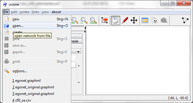
The usual way to get a network into visone is to read it from a local file via the menu file, open
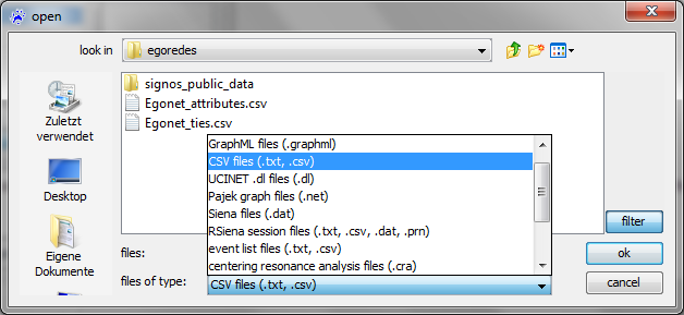
The usual file type to be read by visone is GraphML; GraphML files contain information about nodes and links, about attributes of nodes and links, and about graphical information such as layout, color, or shape. To read GraphML files you select .graphml in the file open dialog (shown below) and click on ok; this is simple, fast, and reliable.
Here, for illustration, we go the hard way and assume that the data are not stored in a GraphML file but in comma-separated-value tables. This very primitive file type can be output from many programs, including statistical software, spread-sheet editors, or other network analysis software. Sometimes you have to deal with this file type.
To open a network from an adjacency matrix file you select files of type CSV files (.txt, .csv) in the file open dialog, select the appropriate file in the file browser, and click on ok. To follow the steps outlined in this tutorial, select the file Egonet_ties.csv.
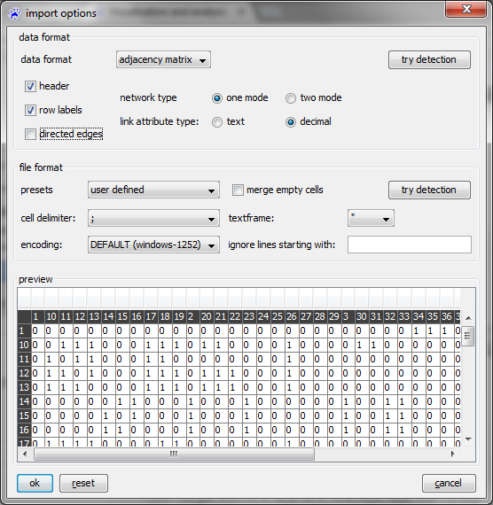
Clicking on ok does not immediatelly open the file. Indeed, in contrast to GraphML, CSV files don't have a self-explaining interpretation; rather the program that has to handle them needs some guidance. Therefore visone opens an import options dialog (see below).
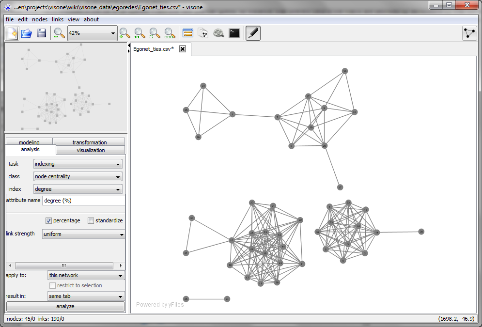
For an exhaustive explanation of all options and their meaning see the page on the import options dialog. To continue with this tutorial, set all options as shown in the image above and click on ok. This opens a network looking like this.
The .csv does not contain layout information. The position of the nodes has been determined by the layout algorithm that can be initiated with the quick layout button.
Apart from GraphML and CSV format, visone can also open files in UCINET's .dl format, in Pajek's .net format, and some more.
A more exhaustive treatment about the various possibilities to import data into visone is given in the data input tutorial.
Importing attributes from CSV tables
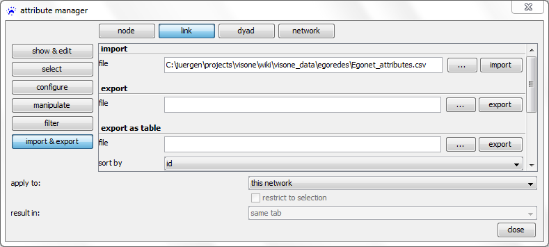
Currently, the nodes have only one attribute called id. The values of other attributes are provided in the file Egonet_attributes.csv. This file can be merged into our current network via the attribute manager which can be started by clicking on the icon ![]() in visone's toolbar.
in visone's toolbar.
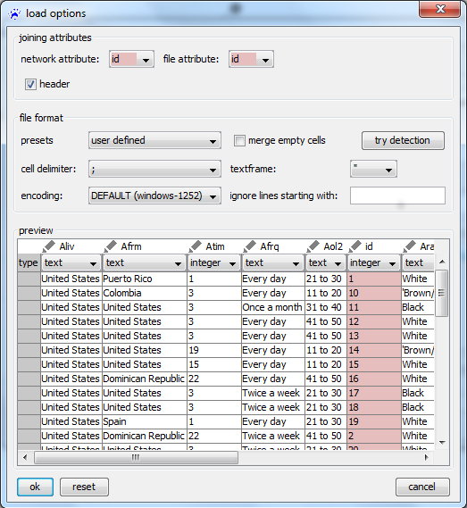
In the attribute manager, choose the node button in the top row, import & export on the left, and select the file Egonet_attributes.csv that you have previously downloaded to your computer as import file. Clicking on import opens a load options dialog similiar to the one below.
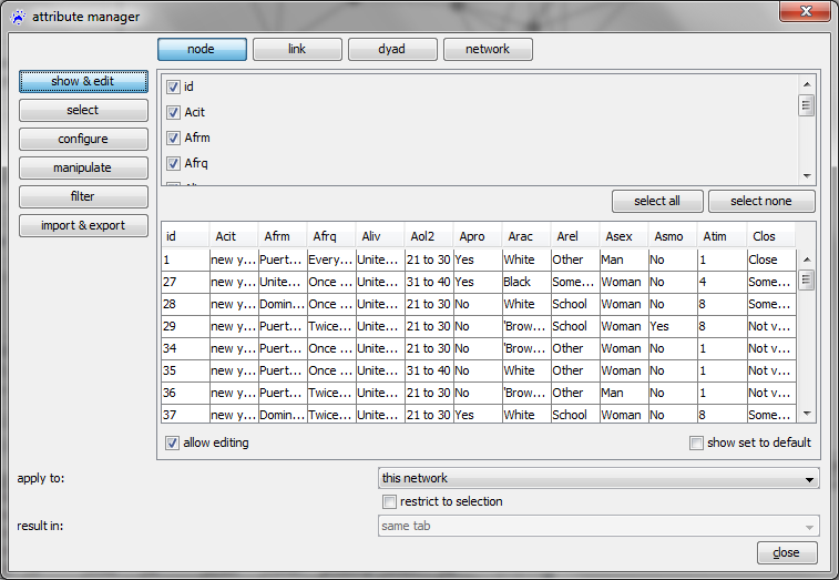
It is very important to set the values of the joining attributes correctly. They should point to the name of the attribute that identifies the nodes (network attribute) and tells visone which column in the imported CSV file holds these identifiers (file attribute). Currently in both drop-down menus id is selected, but in general there might be several node attributes and the nodes could as well be identified by attributes having a different name than id. Setting also the other options as shown above - in particular, setting the cell delimiter to semicolon (;) - and clicking on ok imports the attributes. You can see the result by clicking the show & edit button on the left hand side of the attribute manager. Then, you should see something similar to the following image.
Mapping attributes to graphics: categorical attributes
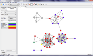
For many networks it is extremly insightful to show the attribute values in the network image. In visone, attributes can be mapped to graphical variables via the visualization tab.
In the visualization tab you can choose between plenty of options; these have to be set from top to bottom. For the category chose mapping since we want to map existing attributes to graphical variables. (The other options are layout for applying a visualization algorithm, geometry for doing affine transformations, such as rotating or scaling, background for setting the background color/image and appearance to attribute for storing x,y coordinates in (new) attributes.)
The type of the mapping refers to the type of the graphical variable that is used for encoding attribute values. This choice is restricted by the type of the attribute that is to be mapped. Numerical attributes can be mapped to graphical variables that allow the user to recognize that one actor has a larger value than another one; examples of such variables are size or position whose usage is demonstrated further down in this tutorial. In this section, however, we want to encode a categorical variable - more specifically, the country of origin of the actor. A good choice for a graphical variable to encode this information is color which we select in the drop-down menu right of type. For property chose node color.
The drop-down menu right of node value should be set to the name of the attribute that is to be encoded; we chose Afrm (meaning country of origin of the actor). Finally, selecting color table for the method option presents you a table with the different values of the Afrm attribute together with a predefined choice of colors that you can change as you wish. Clicking on the visualize button at the bottom of the visualization tab applies the mapping whose result is shown in the network area of the visone window.
Computing network analytic indicators: centrality
visone offers you a rich choice of methods that compute analytic measures on a given network. In this section, we exemplarily compute a centrality indicator on the set of actors. (Node centralities specify which actors are the important ones with respect to a certain criterion.)
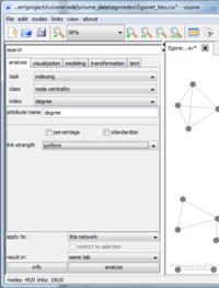
Computing such indicators is done via the analysis tab. To compute the degree of the actors (i.e., the number of ties attached to each actor) set task to indexing. Indexing means that we are assigning values to individual elements (i.e., to nodes or edges) of the network. Set class to node centrality and index to degree. The values specified for link length and link strength can currently only be uniform since we don't have any tie weights. Unchecking the percentage and standardize boxes ensures that the actual degrees are computed. The text field right of attribute name specifies the name of the attribute in which the computed values are to be stored. (visone makes suggestions for this name; at the moment it should say degree but you can change this if you want.)
Having set all these options click on the analyze button at the bottom of the analysis tab. (You won't see any change in the image of the network; however, at the bottom line of the main window visone tells you what has been computed and in which attribute it has been stored.)
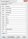
You could browse the values of the newly computed attribute in the attribute manager or in the attributes tab of the node properties dialog (e.g. if you select the node with id 20 you see the last entry telling you that the degree of the node equals 9). You could also export the attributes via the attribute manager (which works similar to the import of attributes explained above) and store them in CSV tables.
However, in many situation it is more insightful to visualize the computed centrality values. This is illustrated in the next section of this tutorial.
Mapping attributes to graphics: numerical attributes
Centrality values (such as the node degrees that have been computed above) are numerical attributes. These can be mapped to graphical variables that let the user distinguish between larger and smaller. Examples of such graphics are size, position (x/y-coordinates), or color gradient. For instance, to map the node degree to the node size you can proceed similar as for mapping categorical attributes (illustrated above). In the visualization tab choose category=mapping, type=size, property=node area, and for attribute=degree; click on visualize.
Network layout
Network layout algorithms compute the positions of nodes, links, and/or labels to yield nice network images. For convenience, a general-purpose layout algorithm can be initiated by clicking on the quick layout button ![]() in visone's toolbar. All other layout algorithms can be initiated from the visualization tab (select category=layout). More explanation can be found in the page on the visualization tab.
in visone's toolbar. All other layout algorithms can be initiated from the visualization tab (select category=layout). More explanation can be found in the page on the visualization tab.
Selecting elements dependent on attribute values
Finally, we demonstrate how network elements (i.e., nodes and links) that have specific attribute values can be selected. Therefore, download the file Egonet.graphml (see the description on the page Egoredes (data)), save it to your computer, and open it in visone via the menu file, open.
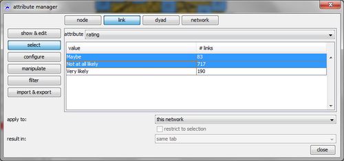
This network turns out to be one big mess containing 45 nodes and 990 links (a simple calculation tells you that the network is complete, i.e., each pair of nodes is connected by a link). The information about which actors actually know each other is encoded in the link attribute rating which can assume the values Not at all likely, Maybe, or Very likely. To delete all links that are not rated as Very likely (say), open the attribute manager, click on the button link in the top, and select on the left-hand side, select the link attribute rating in the drop-down menu. The table shows the different values of this attribute along with the number of links that are assume this value and clicking on one or several rows selects these links. The selected links can be deleted either from the link context menu or from the menu links, delete links. Selecting and deleting those links that are rated as Not at all likely, or Maybe and layouting the network via the quick layout button shows you a network that is identical to the one encoded in the adjacency matrix Egonet_ties.csv.
More sophisticated ways to select network elements are illustrated in the next tutorial on advanced attribute management.
