RSiena (tutorial): Difference between revisions
No edit summary |
|||
| (49 intermediate revisions by 2 users not shown) | |||
| Line 1: | Line 1: | ||
This [[ | This [[Tutorials|tutorial]] illustrates how to analyze longitudinal network data by using [[RSiena | RSiena]] from within visone. We assume that you have installed R on your computer and configured the R connection as it is explained in the [[Installation_(tutorial)#Installing_the_R_connection|installation tutorial]]. We also assume that you have basic understanding about how to work with visone as it is, for instance, explained in the tutorial on [[Visualization_and_analysis_(tutorial)|visualization and analysis]] and basic knowledge of [http://www.stats.ox.ac.uk/~snijders/siena/SnijdersSteglichVdBunt2009.pdf stochastic actor-oriented models (SOAM)]. | ||
To follow the steps illustrated in this | To follow the steps illustrated in this tutorial you should download the file [[Media:Classroom_graphmls.zip|Classroom_graphmls.zip]] and extract (unzip) its content (consisting of the network files <code>classroom_graph1.graphml</code> to <code>classroom_graph4.graphml</code>) to your hard disk. These files constitute the longitudinal network data explained on page [[Knecht_Classroom_(data)|Knecht Classroom (data)]]. | ||
You find all the RSiena functionalities on the '''modeling''' tab on the right side of the visone window selecting ''siena'' in the '''modeling''' drop-down list. Note that first of all the longitudinal network data to be analysed has to be specified as described in the following paragraphs. | |||
To | ==Defining longitudinal network data== | ||
Stochastic Actor Oriented Models (SAOMs) are designed for analysing longitudinal network data given as network panel data, i.e., a sequence of networks representing one network observed at several moments in time. | |||
Such network panel data are encoded in files <code>classroom_graph1.graphml</code> to <code>classroom_graph4.graphml</code>. To load them click on the menu '''file, open''', navigate in the file browser to the directory where you've put the files <code>classroom_graph1.graphml</code> to <code>classroom_graph4.graphml</code> and select all of them before you click the '''ok''' button. (Selection of these files can be done in different ways, for instance, by keeping the '''Control'''-key pushed while successively selecting the files with a mouse left-click or by clicking on one of the files and then typing '''Control-a''' to select all files in the current directory.) | |||
The four networks should be shown in four separate tabs in the [[GUI#network_area|network area]]. However, visone does not yet know that they belong together as a longitudinal network. This information must be given by combining them to a [[network collection]] which is a collection or sequence of several networks that belong together, e.g., by building a longitudinal network. Basic application scenarios related to network collections are explained in the [[Collections_(tutorial)|tutorial on network collections and dynamic networks]]. | |||
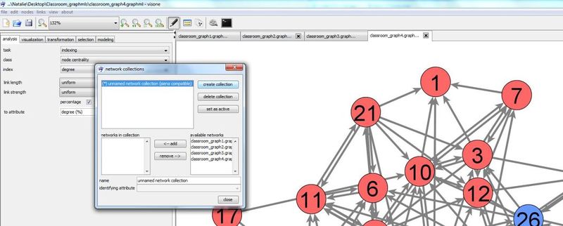
A [[network collection]] can be defined in the [[collection manager | network collection manager]]. To open the [[collection manager | network collection manager]] press button [[File:Collection_manager.png|link=collection_manager]] in [[GUI#toolbar|visone's toolbar]] | |||
[[File:Collection_manager_1.jpg|800px]] | |||
Press '''create collection''' button to create a new collection. A new collection is named 'unknown network collection' by default. You can change the name by clicking in the editable field '''name''' and typing a new one. | |||
[[File:Collection_manager_2.jpg|thumb|250px]] | |||
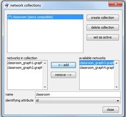
In the right table '''available networks''' all networks that can be added to the selected network collection (the selected collection is indicated by the blue background) are listed. These are basically all currently open networks. Select one of them by clicking at its name and press '''<- add''' to add it to the seleted collection. The table '''networks in collection''' shows you all networks so far contained in the currently selected collection. Note that the top-down order in this table determines the order of the networks in the network collection, hence, has to correspond with their temporal order in the longitudinal network. If the current order is not as you want it, you can rearrange it by removing networks from the collection (clicking at their name and press '''remove ->''') and adding them again which will position them at the very end of the collection. | |||
To follow this tutorial connect <code>classroom_graph1.graphml</code> to <code>classroom_graph4.graphml</code> (in this order) to a network collection named ''classroom'' and set this new collection as active. | |||
Visone knows now the networks that belong to the collection and their order but it does not know which node in the different networks correspond to each other, i.e., represent the same actor at different moments in time. This information has to be given by specifying an [[Identifying_attribute|identifying attribute]]. Candidates for being the identifying attribute are node attributes that are defined in all networks included in the collection. Further they have to be attributes that assign a unique value to each node in a network, i.e., there must not be two nodes in the same network with the same value in those attributes. Among the networks in the network collection nodes with the same value of the identifying attribute are identified with each other. | |||
[[File:Collection_manager_3.jpg|thumb|250px]] | |||
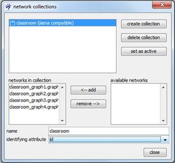
The drop-down list '''identifying attribute''' offers you all available attributes for the current selection that meet the necessary conditions to serve as an identifying attribute. | |||
Note that in the current example you are only offered to choose ''id'' as the identifying attribute as all other attributes do not provide unique values for all nodes in a network. | |||
While you can create a network collection even if some nodes are not present at all time points, a network collection is marked as being '''siena compatible''' if all nodes are present at all times. If a network collection is not siena compatible it cannot be modeled with [[RSiena_interface|RSiena]] but you can nevertheless compute a dynamic layout. | |||
More than one network collection can be created. The analysis with RSiena, however, works on only one longitudinal network data, namely the data represented by the '''active network collection'''. At each moment, only one collection can be active which is indicated by the asterisk '''(*)''' in front of its name. You can switch the active collection with the '''set as active''' button in the collection manager. | |||
==Adding individual or dyadic covariates== | |||
[[File:covariates.jpg|thumb|300px]] | |||
As mentioned before, you find the RSiena functionalities on the '''modeling''' tab on the right side of the visone window where you select ''siena'' in the '''modeling''' drop-down list to get to the '''data specification''' tab. | |||
The '''data specification''' tab offers you a list of all node attributes and dyad attributes that are defined in the first network of the active network collection and can be used as exogenous covariates in the model. | |||
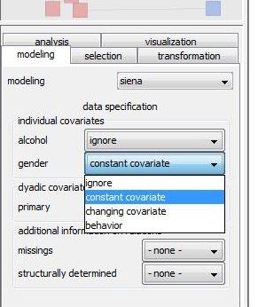
As you see in the right graphic, each attribute name is associated with a drop-down list that contains a choice of covariate types. Actually, this list contains exactly those covariate types that could be represented by the corresponding attribute depending on following conditions: | |||
- an attribute may represent a '''constant covariate''' if it is defined in the first network of the collection. In this case, the attribute values in the first network are assumed to be the values of the constant covariate in the siena model even if the attribute values in the other networks of the collection differ from the values in the first network. | |||
- an attribute may represent '''changing covariate''' if it is defined all but the last network of the collection. It can also be defined in the last network but it is not mandatory as covariates of the last network have no influence on the modeling anyway. Hence, in a network collection that consists of only two networks no changing covariate can be defined. | |||
Especially for node attributes, an additional choice '''behavior''' might be available. If you you select this option, the node attribute will not represent an exogenous covariates but will be treated (together with the network) as a dependent variable that will be modeled itself. | |||
- a node attribute may represent a '''behavior variable''' if it is defined in all networks of the collection and it is of type ''integer'' (You can check and possibly change the ''type'' of an attribute in the attribute manager under configurations) | |||
Specify for all attributes which type of covariate they should define or whether they should not be inluded (by selecting ''ignore'') in the model. | |||
To follow this tutorial set ''gender'' as constant individual covariate and ''primary'' as constant dyadic covariate. | |||
==Specifying missing data or structurally fixed values== | |||
==Model specification and estimation== | |||
After the data specification (networks, behavior variables, covariates, missing data, structurally fixed values) is complete, the model can specified. To do so, visone provides the '''model specification''' dialogue which you open by pressing the '''specify model''' button at the bottom of the '''siena modeling''' tab. | |||
[[File:modelspecification.jpg|600px]] | |||
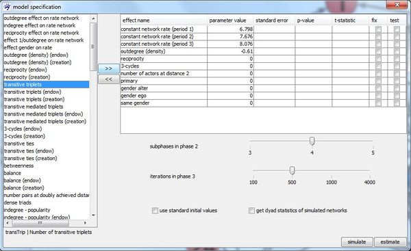
The left list in this dialogue contains all effects (if you do not know what ''effect'' in this context means, see the [http://www.stats.ox.ac.uk/~snijders/siena/SnijdersSteglichVdBunt2009.pdf tutorial] on stochastic actor-oriented models) that are available for the active network collection with the above specified individual and dyadic covariates. For instance, we find the covariate related effect ''primary'' that takes the influence of having been together in the same primary school on the existence of a network tie into account. This effect would not have been in the list of available effect if we had not set ''primary'' as a dyadic attribute. Also the actor covariate related effects ''gender ego'',''gender alter'', and ''same gender'' can be added to the model only because we included gender as an individual covariate. | |||
An available effect can be added to the model by selecting it (i.e., clicking at its name in the left list) and pressing button '''>>''' on the right side of the list. Immediately, the effect name disappears from the left list and appears in the right table which contains all effects that are currently included in the model. If you want do exclude an effect already included effect from the model, select it in the right table and press '''<<'''. | |||
By ticking checkbox '''use standard initial values''' it can be set whether standard values or current parameter values shall be used as initial values in the estimation process. Furthermore, the number of subphases in the parameter estimation phase (''phase 2'') and the number of iterations in the standard error estimation phase (''phase 3'') (see the [http://www.stats.ox.ac.uk/~snijders/siena/RSiena_Manual.pdf RSiena manual]) can be set by shifting the corresponding sliders. | |||
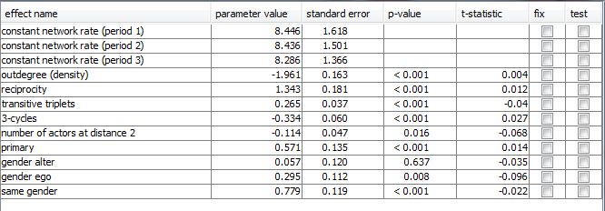
You start the parameter estimation by pressing button '''estimate'''. The estimation progress can be monitored in the ''Rserve'' window (console). When the estimation is finished, the results are displayed in the right table of the model specification dialogue. | |||
[[File:estimates.jpg|700px]] | |||
For each included effect its estimated '''parameter value''', associated '''standard error''', and '''t-statistic''' (that | |||
indicates the convergence of the estimation process, see the [http://www.stats.ox.ac.uk/~snijders/siena/RSiena_Manual.pdf RSiena manual]) are displayed. The '''p-value''' assumes the null hypothesis that respective parameter values is 0 and is computed by | |||
the R command 2*pnorm(-abs(parameter estimates/standard errors)). | |||
It is also possible to test or fix certain effects by ticking the correspondig checkboxes. | |||
When an effect was tested, its p-value results from the score-type test as described in the[http://www.stats.ox.ac.uk/~snijders/siena/RSiena_Manual.pdf manual]. | |||
When the '''model specfication''' dialogue is closed, he has the possibility to save the | |||
RSiena output file is offered. This file contains the standard RSiena-output for estimation results. | |||
==Simulation== | |||
It is also possible to simulate networks based on model predictions. By pressing the simulate button a number of networks is simulated based on current model specification and parameter estimates. The number of simulated networks equals the number of iterations in phase 3 as set by the user. For each pair of actors the average number of being linked in this simulations is calculated. The resulting ''tie probabilities'' are saved as an dyad attribute named '''tie probabilities'''. | |||
==Visualize simulated netwoks== | |||
Latest revision as of 14:56, 18 July 2012
This tutorial illustrates how to analyze longitudinal network data by using RSiena from within visone. We assume that you have installed R on your computer and configured the R connection as it is explained in the installation tutorial. We also assume that you have basic understanding about how to work with visone as it is, for instance, explained in the tutorial on visualization and analysis and basic knowledge of stochastic actor-oriented models (SOAM).
To follow the steps illustrated in this tutorial you should download the file Classroom_graphmls.zip and extract (unzip) its content (consisting of the network files classroom_graph1.graphml to classroom_graph4.graphml) to your hard disk. These files constitute the longitudinal network data explained on page Knecht Classroom (data).
You find all the RSiena functionalities on the modeling tab on the right side of the visone window selecting siena in the modeling drop-down list. Note that first of all the longitudinal network data to be analysed has to be specified as described in the following paragraphs.
Defining longitudinal network data
Stochastic Actor Oriented Models (SAOMs) are designed for analysing longitudinal network data given as network panel data, i.e., a sequence of networks representing one network observed at several moments in time.
Such network panel data are encoded in files classroom_graph1.graphml to classroom_graph4.graphml. To load them click on the menu file, open, navigate in the file browser to the directory where you've put the files classroom_graph1.graphml to classroom_graph4.graphml and select all of them before you click the ok button. (Selection of these files can be done in different ways, for instance, by keeping the Control-key pushed while successively selecting the files with a mouse left-click or by clicking on one of the files and then typing Control-a to select all files in the current directory.)
The four networks should be shown in four separate tabs in the network area. However, visone does not yet know that they belong together as a longitudinal network. This information must be given by combining them to a network collection which is a collection or sequence of several networks that belong together, e.g., by building a longitudinal network. Basic application scenarios related to network collections are explained in the tutorial on network collections and dynamic networks.
A network collection can be defined in the network collection manager. To open the network collection manager press button ![]() in visone's toolbar
in visone's toolbar
Press create collection button to create a new collection. A new collection is named 'unknown network collection' by default. You can change the name by clicking in the editable field name and typing a new one.
In the right table available networks all networks that can be added to the selected network collection (the selected collection is indicated by the blue background) are listed. These are basically all currently open networks. Select one of them by clicking at its name and press <- add to add it to the seleted collection. The table networks in collection shows you all networks so far contained in the currently selected collection. Note that the top-down order in this table determines the order of the networks in the network collection, hence, has to correspond with their temporal order in the longitudinal network. If the current order is not as you want it, you can rearrange it by removing networks from the collection (clicking at their name and press remove ->) and adding them again which will position them at the very end of the collection.
To follow this tutorial connect classroom_graph1.graphml to classroom_graph4.graphml (in this order) to a network collection named classroom and set this new collection as active.
Visone knows now the networks that belong to the collection and their order but it does not know which node in the different networks correspond to each other, i.e., represent the same actor at different moments in time. This information has to be given by specifying an identifying attribute. Candidates for being the identifying attribute are node attributes that are defined in all networks included in the collection. Further they have to be attributes that assign a unique value to each node in a network, i.e., there must not be two nodes in the same network with the same value in those attributes. Among the networks in the network collection nodes with the same value of the identifying attribute are identified with each other.
The drop-down list identifying attribute offers you all available attributes for the current selection that meet the necessary conditions to serve as an identifying attribute. Note that in the current example you are only offered to choose id as the identifying attribute as all other attributes do not provide unique values for all nodes in a network.
While you can create a network collection even if some nodes are not present at all time points, a network collection is marked as being siena compatible if all nodes are present at all times. If a network collection is not siena compatible it cannot be modeled with RSiena but you can nevertheless compute a dynamic layout.
More than one network collection can be created. The analysis with RSiena, however, works on only one longitudinal network data, namely the data represented by the active network collection. At each moment, only one collection can be active which is indicated by the asterisk (*) in front of its name. You can switch the active collection with the set as active button in the collection manager.
Adding individual or dyadic covariates
As mentioned before, you find the RSiena functionalities on the modeling tab on the right side of the visone window where you select siena in the modeling drop-down list to get to the data specification tab. The data specification tab offers you a list of all node attributes and dyad attributes that are defined in the first network of the active network collection and can be used as exogenous covariates in the model.
As you see in the right graphic, each attribute name is associated with a drop-down list that contains a choice of covariate types. Actually, this list contains exactly those covariate types that could be represented by the corresponding attribute depending on following conditions: - an attribute may represent a constant covariate if it is defined in the first network of the collection. In this case, the attribute values in the first network are assumed to be the values of the constant covariate in the siena model even if the attribute values in the other networks of the collection differ from the values in the first network. - an attribute may represent changing covariate if it is defined all but the last network of the collection. It can also be defined in the last network but it is not mandatory as covariates of the last network have no influence on the modeling anyway. Hence, in a network collection that consists of only two networks no changing covariate can be defined.
Especially for node attributes, an additional choice behavior might be available. If you you select this option, the node attribute will not represent an exogenous covariates but will be treated (together with the network) as a dependent variable that will be modeled itself. - a node attribute may represent a behavior variable if it is defined in all networks of the collection and it is of type integer (You can check and possibly change the type of an attribute in the attribute manager under configurations)
Specify for all attributes which type of covariate they should define or whether they should not be inluded (by selecting ignore) in the model.
To follow this tutorial set gender as constant individual covariate and primary as constant dyadic covariate.
Specifying missing data or structurally fixed values
Model specification and estimation
After the data specification (networks, behavior variables, covariates, missing data, structurally fixed values) is complete, the model can specified. To do so, visone provides the model specification dialogue which you open by pressing the specify model button at the bottom of the siena modeling tab.
The left list in this dialogue contains all effects (if you do not know what effect in this context means, see the tutorial on stochastic actor-oriented models) that are available for the active network collection with the above specified individual and dyadic covariates. For instance, we find the covariate related effect primary that takes the influence of having been together in the same primary school on the existence of a network tie into account. This effect would not have been in the list of available effect if we had not set primary as a dyadic attribute. Also the actor covariate related effects gender ego,gender alter, and same gender can be added to the model only because we included gender as an individual covariate.
An available effect can be added to the model by selecting it (i.e., clicking at its name in the left list) and pressing button >> on the right side of the list. Immediately, the effect name disappears from the left list and appears in the right table which contains all effects that are currently included in the model. If you want do exclude an effect already included effect from the model, select it in the right table and press <<.
By ticking checkbox use standard initial values it can be set whether standard values or current parameter values shall be used as initial values in the estimation process. Furthermore, the number of subphases in the parameter estimation phase (phase 2) and the number of iterations in the standard error estimation phase (phase 3) (see the RSiena manual) can be set by shifting the corresponding sliders.
You start the parameter estimation by pressing button estimate. The estimation progress can be monitored in the Rserve window (console). When the estimation is finished, the results are displayed in the right table of the model specification dialogue.
For each included effect its estimated parameter value, associated standard error, and t-statistic (that indicates the convergence of the estimation process, see the RSiena manual) are displayed. The p-value assumes the null hypothesis that respective parameter values is 0 and is computed by the R command 2*pnorm(-abs(parameter estimates/standard errors)). It is also possible to test or fix certain effects by ticking the correspondig checkboxes. When an effect was tested, its p-value results from the score-type test as described in themanual.
When the model specfication dialogue is closed, he has the possibility to save the RSiena output file is offered. This file contains the standard RSiena-output for estimation results.
Simulation
It is also possible to simulate networks based on model predictions. By pressing the simulate button a number of networks is simulated based on current model specification and parameter estimates. The number of simulated networks equals the number of iterations in phase 3 as set by the user. For each pair of actors the average number of being linked in this simulations is calculated. The resulting tie probabilities are saved as an dyad attribute named tie probabilities.
