Data input (tutorial)

Normally, visone reads network data from GraphML files, which should never cause any problems. However, in some cases it is necessary to import data stemming from other sources that can, for instance, export adjacency matrices to comma-separated-value (CSV) tables. This tutorial guides you through the various possibilities to input data into visone.

The usual way: read GraphML

GraphML is the usual file format for visone; it encodes the three types of information that are contained in visone networks: network structure, attributes, and graphical information and it is the only format that does so. To read network data from GraphML files use the file menu, click on open..., select files of type .graphml, and click on the ok button.

The other file types are only needed when you want to import data from other sources that cannot output GraphML.

An overview about the other possibilities

Apart from GraphML, visone can read network data from files that are exported by other network analysis software, including UCINET, Pajek, Siena, and some more. Opening these files is also done via the file menu by selecting the appropriate file type. More information about reading these file types is provided in the section about other supported formats.

A more basic option that should be feasible in most situations is to read network data from comma-separated-value (CSV) files. CSV files are plain-text files, for example looking like this

  ;A;B;C;D
 A;0;1;1;1
 B;1;0;1;0
 C;1;1;0;0
 D;1;0;0;0

that can be created by spread sheet editors (such as MS Excel), statistical software, most network analysis software, and many more. However, reading data from CSV files is more error-prone since these files do not come with an unequivocal definition about how to interpret them (rather you have to tell the program how these files should be interpreted). Most of this tutorial is dedicated to the import of CSV files.

Personal networks collected with the EgoNet software can be converted to GraphML with the EgoNet2GraphML converter. This is illustrated in the tutorial on personal networks.

Wikipedia edit networks can be imported after converting edit history files with the WikiEvent software. This is illustrated in the tutorial on Wikipedia edit networks.

If nothing else works, you can make use of the visone R console that allows access to the R environment for statistical computing or you can read data via the KNIME connection that connects visone to a comprehensive data mining workflow tool. Both environments, R and KNIME, provide very general and configurable methods for data input and, in addition, enable you to preprocess and/or filter the data with relatively low effort. We provide more information about these possibilities in the section "if nothing else works".

Yet another possibility to create networks directly in visone is to enter them manually (which is only appropriate if the neworks are small and the data is not yet available in electronic format). This option is illustrated in the tutorial introducing the visual network editor.

The variants of comma-separated-value (CSV) files

A comma-separated-value file can be thought of as a plain-text file that encodes a table, i.e., a data array that has rows and columns - sometimes also referred to as a matrix. In a network context, there are different possibilities to encode information about nodes, links, or attribute information in such tables. The first three (adjacency matrices, link lists, and adjacency lists) provide information about nodes and links and can be opened via the file menu by selecting the appropriate file type. Attribute tables provide information about node or link attributes and can be opened via the attribute manager. What follows is a short characterization of these file types; more exhaustive explanation about how to read them is given in the following sections.

Adjacency matrix files. An adjacency matrix encodes for all pairs of nodes (indexing the rows and columns of the table) whether or not there is a link connecting these nodes. An example is shown in the following.

  ;A;B;C;D
 A;0;1;1;1
 B;0;0;1;0
 C;1;1;0;0
 D;1;0;0;0

The first row and the first column are the labels of the nodes; the remaining part encodes whether there is a link from the node indexing the row to the node indexing the column. For instance, the character 1 in the row indexed by A and the column indexed by B indicates that there is a link going from A to B; the 0 in the row B and column A indicates that there is no link in the reverse direction.

Link list files. A link list contains as many rows as there are links in the network and (in its most basic form) a link list contains two columns where the entry in the first column is the identifier for the source node and the entry in the second column denotes the target node of the link. The following example

 A;C
 C;B
 B;A
 A;D

defines four links: from node A to node C, from C to B, etc. Note that link lists use less space than adjacency matrices - especially if the network is very sparse (i.e., when the number of links divided by the number of node pairs is a small value close to zero).

Adjacency list files. An adjacency list has as many rows as there are nodes in the network. Each row may have a different length and the row associated with a node lists all neighbors of this node. For instance, in the following example

 A;2;3;1
 B;0;2
 C;1;0
 D;0

the labels at the beginning of each row are the node identifiers (these ids are optional); A is the label of the node with index 0, B is the label of the node with index 1, etc; the list 2;3;1 following the label A defines that there are links from A to the node with index 2 (labeled C), to the node with index 3 (D), and to the node with index 1 (B).

Attribute tables. An attribute table has one row that lists the attribute names (in the example below this is id;age;smokes followed by as many rows as there are nodes in the network.

 id;age;smokes
 A;23;false
 B;28;true
 C;19;true
 D;27;false

One of the columns (id in the example above) lists the unique node identifiers (it is not necessarily the first row and not necessarily labeled id). The other columns list the attribute values of the attribute whose name is given in the respective column header. Attribute files are not read via the file menu but can only be added to an existing network via the attribute manager.

Note: visone does not allow to simultaneously input an adjacency matrix together with given attributes in one file. That is, a file like

  ;A;B;C;D;age;smokes
 A;0;1;1;1;23;false
 B;1;0;1;0;28;true
 C;1;1;0;0;19;true
 D;1;0;0;0;27;false

(having the interpretation that the first four columns specify an adjacency matrix and the last two columns define node attribute values) cannot be opened. Rather you have to split this into two separate files, one containing the adjacency matrix which can be opened via the file menu and the other containing the attribute table which can be opened via the attribute manager. (For instance, in MS Excel you could split the file by selecting columns, copy them, and past them into a new table.)

The next four sections explain the various options that have to be set when reading CSV files.

Adjacency matrix files

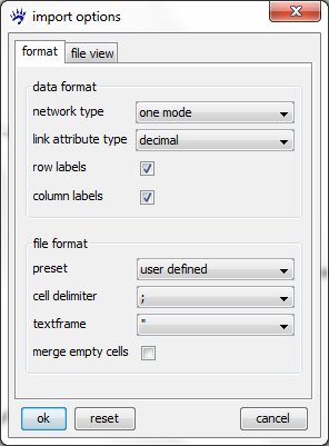
To open an adjacency matrix, use the file menu, click on open..., select files of type adjacency matrix files (.txt, .csv) in the file chooser, navigate to the file you want to open, and click on the ok button. Then the import options dialog opens (show below).

The import options dialog has two tabs labeled format where you can set the various options and file view where you can see the contents of the file. The semantics of the various options is explained in the following.

• network type can be one mode or two mode. In the adjacency matrix of a one mode network the rows and columns are indexed by the same set of nodes; for a two mode network (for instance, a network connecting authors to the articles they have written), the rows and columns are indexed by different sets of node (authors respectively articles in the above example).
• link attribute type can be decimal or text. The entries of the adjacency matrix (which are either numbers or character strings) are saved in a link attribute of the newly opened network; this option defines the type of this attribute (decimal for numerical attributes and text for categorical).
• The check boxes row labels and column labels indicate whether the first row (respectively first column) lists the node identifiers (rather then entries of the adjacency matrix). If unchecked, then the node identifiers will be the numbers from $0$ to $n-1$ (when there are $n$ nodes in the network).
• The file format can be MS Excel, OpenOffice (default CSV output of these software programs, respectively), or user defined. If it is set to user defined you have to specify the following options.
• cell delimiter defines the character that separates one matrix cell from the next. In the examples above, the cell delimiter was always the semicolon (;) but it can as well be a comma, colon, TAB, or SPACE character.
• textframe can be double quotes, quotes, or NONE. Textframes are necessary if the matrix-cell entries themselves contain the cell delimiter. (For instance, if the cell delimiter is SPACE and the row/column labels are "firstname lastname"; the quotes tell visone that the cell does not end after firstname.)
• The merge empty cells checkbox tells visone whether repeated cell delimiters should be treated as one. This option is for instance necessary when reading the Newcomb Fraternity data (of which an excerpt is shown below)

  0  7 12 11 10  4 13 14 15 16  3  9  1  5  8  6  2
  8  0 16  1 11 12  2 14 10 13 15  6  7  9  5  3  4
 13 10  0  7  8 11  9 15  6  5  2  1 16 12  4 14  3
 ...

where the cell delimiter (the SPACE character) is sometimes repeated to enhance (human) readability.

When you have set the options, click on the ok button to open the file.

Link list files

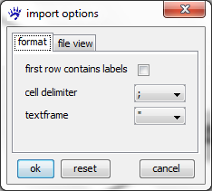
To open a link list, use the file menu, click on open..., select files of type link list files (.txt, .csv) in the file chooser, navigate to the file you want to open, and click on the ok button. Then the import options dialog opens (show below).

The checkbox first row contains labels indicates whether the first row lists the attribute names of the link attributes encoded in the table (rather than the node pairs and attribute values). In the example below, each link (defined by its two endpoints nodeID1 and nodeID2 has two attributes: a link id which are just the numbers from 1 to n and a type which has in our example the values friend or enemy.

 nodeID1;nodeID2;id;type
 A;C;1;enemy
 C;B;2;friend
 B;A;3;enemy
 A;D;4;friend

The other options have the same meaning as when reading adjacency matrices (explained above).

Adjacency list files

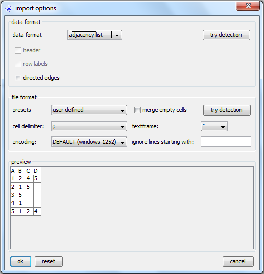
To open an adjacency list, use the file menu, click on open..., select files of type adjacency list files (.txt, .csv) in the file chooser, navigate to the file you want to open, and click on the ok button. Then the import options dialog opens (show below).

• The header checkbox defines whether the first row is a header giving the numbers of nodes and links in the file (rather then the adjacency list of the first node).
• node labels indicates whether the first column list the node identifiers (if unchecked, then nodes are numbered consecutively and the $i$'th row list the neighbors of the $i$'th node).
• directed defines links are treated as directed or undirected.

The other options have the same meaning as when reading adjacency matrices (explained above).

Importing node and link attributes

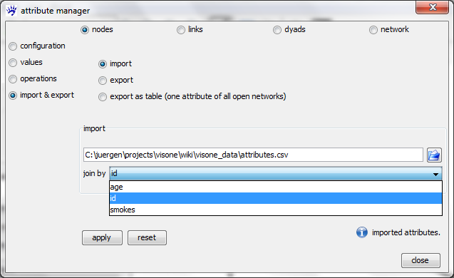
To open an attribute table and add attribute values to the nodes or links of a network that is already opened in visone, use the attribute manager, select nodes (respectively links) in the radio buttons in the top row, select import & export in the radio buttons on the left hand side, select import, and navigate to the CSV file containing the attribute values. The join by drop-down menu must be set to that node attribute (respectively link attribute) that identifies the nodes (links). In the example below this attribute is named id but it could have any other name. (Note that, in general, age or smokes could not serve as identifying attributes, since their values are not unique.)

The identifying attribute must be identical to the header of the column that contains the identifiers (see below). The other columns contain the names and values of the other attributes. For instance, the node with id A gets a value of 23 for the age attribute and the value false for the smokes attribute. (When reading attribute tables you need column headers.)

 id;age;smokes
 A;23;false
 B;28;true
 C;19;true
 D;27;false

Clicking on the apply button opens the import options which have the same meaning as when reading adjacency matrices (explained above).

If nothing else works: use the R console or KNIME connection

visone offers the R console with which network data can be sent from visone to R and back. This ability to load data from R - together with R's data input and data processing capabilities - opens nearly unlimited possibilities to import data from yet other sources, as well as to import data that has to be cleaned, filtered, or preprocessed before turning it into a network.

The basic functioning of the visone to R interface is explained in the R tutorial. Tutorials about working with R are linked from the R website. A particular useful R package for data input is the foreign package for "reading and writing data stored by statistical packages such as Minitab, S, SAS, SPSS, Stata, Systat, ..., and for reading and writing dBase files."