Event networks (tutorial)

The links in an event network encode time stamped interaction among actors, for instance, users sending emails to other users. There is an important difference to networks of relational states - such as friendship networks. To illustrate the difference, when two actors are friends of each other at some instant in time, then - if nothing happens in between - they are still friends in the very near future. In contrast, if someone sends and email to another person at some instant in time, then he/she does not necessarily send an email to the same person in the very next instant in time. Stated otherwise, relations like friendship have inertia (something has to happen to change them), while relational events mark time points of interaction.

This tutorial is a practically oriented, example based, "how-to" guide illustrating the import, transformation, visualization, and analysis of event networks with visone. More background on event networks can be found in

Carter T. Butts: A Relational event framework for social action. Sociological Methodology 38(1):155-200, 2008.
Ulrik Brandes, Jürgen Lerner, and Tom A. B. Snijders: Networks Evolving Step by Step: Statistical Analysis of Dyadic Event Data. Proc. 2009 Intl. Conf. Advances in Social Network Analysis and Mining (ASONAM 2009), pp.200-205. IEEE Computer Society, 2009.

and in other papers linked in the references.

Please address questions and comments about this tutorial to me (Jürgen Lerner).

Example data: networks of political conflict and cooperation

This tutorial uses for illustration networks of events among political actors that have been collected by the Penn State Event Data Project (formerly Kansas Event Data System). Specifically, we use data encoding events in or around the Persian Gulf region in the time from 1979 to 1999. This data set is described in and linked from the page on Penn State Event Data. To follow the steps outlined in this tutorial you should download the file Gulf_events_preprocessed.zip.

Another specific application area for event networks - using different example data - is treated in the tutorial on Wikipedia edit networks.

Importing event networks

visone can import event lists from comma-separted-value (CSV) files. These files must contain a header in the first line (giving the column labels) followed by any number of lines each of which encodes one event. For instance, some lines in the example file look like this.

 "WEIS.code";"Time";"Source";"Target";"Description";"Goldstein.weight";"Type"
 ...
 222;980213;"ISR";"WES";"NONMIL DESTR";-8.7;"conflict"
 223;920717;"SYR";"ISR";"MIL ENGAGEME";-10;"conflict"
 ...

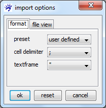
To open such a file, click on open in the file menu, select files of type: event list files (.csv, .txt), navigate to the file that you want to open, and click on ok. In the import options dialog (see below) you have to specify the character that separates the different entries in each line - this is the semicolon (;) in our example file - and a character enclosing text (if any) - this is the double quotes (") in our example file.

To find out the right settings you can look at the file tab in the import options dialog showing you part of the input file.

visone can now read the various entries of the input file - and you have to specify how these should be mapped to the resulting network in the dialog EventNetwork specification (shown below). Concretely you have to specify how the various components of an event are encoded in the file (Event format tab); how to iterate over the network sequence (Event iterator tab); how the events are mapped to the network's link attributes (Event network tab); and, if desired, which statistics should be computed while constructing the event network (Eventnet statistics tab). The tabs should be filled out in the order as they are numbered in the dialog since choice-possibilities for the latter tabs depend on previous settings. If you make changes in some tab you have to subsequently set (again) the values for the latter tabs.

Event format

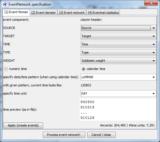
In the event format tab (see the image below) you first have to specify which columns of the input file hold the information about the five components of an event (these are source, target, time, type, and weight). In our example, you can set the values as in the image below. The meaning of the five components is explained in the following.

SOURCE The source actor is the one who initiates the event.
TARGET The target actor is the one who receives the event.
TIME The time denotes when the event happened. visone supports a wide range of time encodings - from numeric times to strings representing calendar date and time in more common or less common formats. Furthermore, a time unit can be specified that defines the precision of the time variable.
TYPE The event type is a categorical variable specifying what happened. In our example, there are different choices for event types. One possibility is the rather coarse distinction between cooperative (positive) and conflictive (negative) events. The other possibility is to distinguish between all more than 100 different WEIS event types. An intermediate possibility (and that's what we are going to do in the following) is to use just the distinction between conflict and cooperation but to distinguish quantitatively between "strong" events and "weak" events by the event weight. For instance, the use of military force is counted more seriously than a warning - even though both are conflictive events.
WEIGHT The event weight is a numeric variable quantifying the intensity of the event with respect to the event type (see the example above). For instance, military engagement has a weight of -10.0 while warnings have a weight of -3.0.

After these five components have been chosen visone needs some information about the interpretation of time. The first choice is the selection between numeric time (if the time fields correspond to integer numbers) or calendar time (if time fields can somehow, specified below, be turned into a date/time). We have calendar time in our example.

If time is given by calendar, a time format pattern has to be specified. visone proposes some known pattern - among others the pattern yyMMdd which is appropriate for the KEDS event times. (This pattern implies that there are two digits for the year, followed by two digits for the month, followed by two digits for the day of the month; for instance, 940930 for September 30, 1994.) You can enter other than the proposed patterns in the textfield if date/time is formatted differently (see the webpage on the java class SimpleDateFormat for guidance). visone assists you in finding the right pattern by showing some date/time strings as they appear in the file and - whenever you select a date format pattern - the dialog shows you the current time formatted by the specified pattern.

Finally, you have to specify a time unit. If time is numeric you have to enter an integer in the textfield. If time is given by calendar you can select a "natural" time unit from Millisecond to Year. An appropriate time unit makes the iteration over the event sequence (and potentially the decay of link attributes over time) more intuitive. When computing event network statistics, events that happen within the same time unit are treated as independent of each other. The time of the KEDS events is given by the day. Thus, appropriate time units are DAY or coarser.

Note that the only required information are the columns containing the source and target - for the other components you can take default values (by selecting <implied> instead of a column header). The default value for the event type is the string EVENT (taking this default type means that there is no variation in event types - all have the same type); the default weight is equal to 1.0; the default event time is the row number in the input file (so that only the order of events is taken into account).

When all settings in the event format tab are done, you can create the list of events by clicking on the Apply (create events) button. A message informs about the number of events and the number of time units from the first to the last event. (The events are sorted in ascending order by time after reading them - thus, it is not necessary that the events are ordered by time in the input file.)

Event iterator

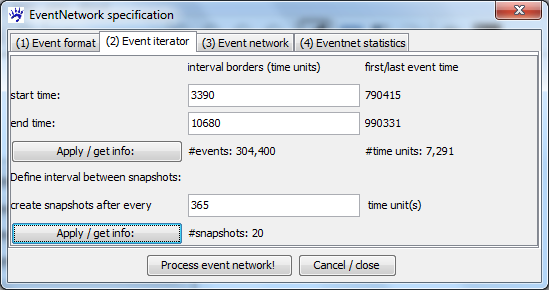
In the event iterator tab (see below) you have to specify the start and end time of the time interval to be processed and the delay between network snapshots.

When the events have been created after filling out the event format tab (see the preceeding section) visone suggests as start time the time of the first event and as end time the time of the last event. If you don't want to process the whole event sequence you can increase the start time and/or decrease the end time. After clicking on the upper Apply / get info button, visone informs you about the number of events and time units in the specified subsequence. You might just take all events by not changing the interval borders; this includes all events from April 15, 1979 to March 31, 1999 - as can be seen in the dialog.

Then you have to choose the time points when a network snapshot is to be created by specifying the delay between snapshots. You can see in the dialog that the event sequence spans more than 7,200 time units (i.e., days with the current settings) which is almost 20 years. The number of snapshots must be small (some 10 or 20 snapshots are ok), since they are all opened in a new tab in visone. When we want to create a snapshot once a year we specify create snapshots after every 365 time unit(s). (The number of snapshots is then 20.) visone always creates one snapshot at the end of the event sequence - even if the waiting time is less than the specified number.

Event network

The tab to specify the event network is the most important one - here you define which link attributes of the event network summarize the past events, how events of various types add to these attributes, and how they change over time.

The first thing to do is to decide on the link attributes. Here you are free to choose any attribute name (that makes it easy to remember the intuition of the attribute). Furthermore, a halftime - defining how fast attributes decay over time - has to be specified. The halftime has the following effect: when a particular link attribute on a particular dyad (pair or actors) has a value of $x$ at time $t$ , then (if no event on the same dyad happens in between) the value is $x/2$ at time $t+halftime$ . Intuitively, link attributes with a positive halftime capture recent interaction; if the halftime gets shorter then they capture even more recent interaction. A halftime equal to zero or negative indicates that the respective attribute does not decay over time; these attributes capture past interaction irrespective of the elapsed time.

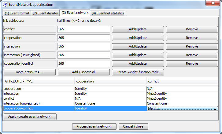
In our concrete example we choose the following link attributes that all have a halftime of (approximately) one year.

An attribute cooperation sums up the weights of past cooperative events.
The link attribute conflict is similar and sums up past conflictive events. This attribute will also be non-negative; that is, a higher value means more past/recent conflict. (See later how this is achieved.)
Interaction sums up the strength of past events - irrespective of whether these are cooperative or conflictive.
Interaction (unweighted) sums up the number of past events - irrespective of whether these are cooperative or conflictive and irrespective of their weight.
Finally cooperation-conflict sums up the (positive) weights of cooperative events and the (negative) weights of conflictive events. This attribute is positive on dyads that have more cooperative events (or cooperative events with higher weights) and it is negative on dyads on which there are more conflictive events (or more serious conflictive events).

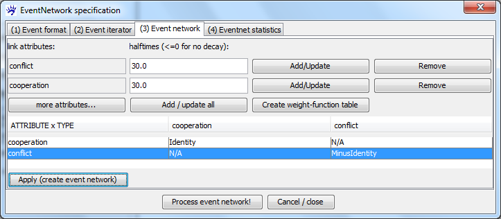
When the link attributes are added (e.g., click on the Add / update all button) you have to specify how the events contribute to them. Clicking on Create weight-function table builds a table that has one row for each link attribute and one column for each event type. In the cell indexed by an attribute $attr$ and an event type $t$ you specify the function mapping weights of events of type $t$ to increments of the link attribute $attr$ . In our example, selecting the function Identity in the cell indexed by attribute cooperation and event type cooperation means that whenever an event of type cooperation and weight $w$ happens then you add $w$ to the current value of the cooperation attribute. If we had chosen SquareRoot as the weight function in the same cell, then we would add ${\sqrt {w}}$ to the cooperation attribute whenever an event of type cooperation and weight $w$ happens. The weight-function identifier N/A means that events of that type do not cause any change of the respective attribute. For instance, events of type conflict do not change the attribute cooperation. Note that for the attribute conflict and the type conflict we choose the weight function MinusIdentity; thus, when a conflictive event with weight -10 happens we add the (positive) value 10 to the attribute conflict (thereby the conflict attribute is always non-negative and higher values indicate more past conflicts). The settings for all attributes and types can be seen in the above image.

After these settings have been done you can create the snapshots by clicking on the button Process event network!. If you want to create a statistics table you first have to fill out the tab number 4. We turn to the statistics later and create the snapshots now.

Visualization and analysis of event networks

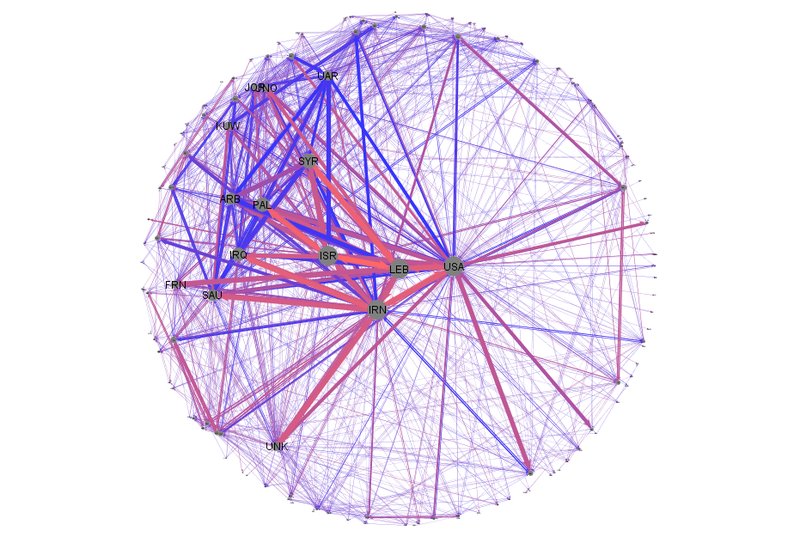
With the above settings visone opens 20 network tabs. The nodes in the network have an attribute label that holds the names of the source or target nodes as they are given in the event list file. The links have (in our example) five numerical attributes encoding the values of the link attribute functions at the time of the snapshot. These link attributes allow to compute, for instance, the total amount of conflict or cooperation received or initialized by the actors (compute the indegree respectively outdegree with link strength set to conflict or cooperation or any other link attribute). These degrees can, for instance, be used for visual filtering by mapping the centrality values to size or color of the nodes or selecting nodes by importance. Examples for visualization of event networks can be found in the tutorial on Wikipedia edit networks. Note that all analysis and visualization tasks can be done in parallel for all open network tabs and note that visone also offers to compute a dynamic layout that can be animated; this is illustrated in the tutorial on network collections. The image below is an example placing the most involved actors in the center of the drawing and coding rather cooperative ties in blue and rather conflictive ties in red.

Statistical modeling of the conditional event type or weight

While importing event networks it is possible to compute and save network statistics associated with dyadic events that can be used to build and estimate a statistical model for the conditional event type. Such models have been proposed in Ulrik Brandes, Jürgen Lerner, and Tom A. B. Snijders (2009): Networks Evolving Step by Step: Statistical Analysis of Dyadic Event Data. These models can be used to test whether the network of past events explains the likelihood that future events among a given pair of actors are rather cooperative or rather conflictive, for instance

Do actors have a tendency to fight those that attacked them in the past? (Tendency to retalliate.)
Do actors have a tendency to cooperated with the enemies of their enemies, to fight the friends of their enemies, etc?

The event network statistics can be computed during importing the data, are saved in a file, and can then be analyzed with any statistical software, such as R.

It is important to understand that with the statistics table computed by visone you can estimate a model for the conditional event type, given that an event happens, as this has been defined in Brandes et al.(2009). With the visone output you cannot model the likelihood that two actors interact at all. (Such models can be specified and fitted, for instance, with the R package relevent.) More on the difference between modeling the conditional event type and the marginal (unconditional) event type can be found in the slides Modeling Frequency and Type of Interaction in Event Networks (.pdf).

To make the analysis comparable to the one presented in Brandes et al.(2009), we modify the link attributes in the event network tab slightly (see below). Specifically we set the halftime to 30 days and include only the attributes conflict and cooperation. (The settings in the event format stay the same and in the event iterator tabs you may set the delay between snapshots to 7291 to create only one snapshot.)

Event statistics

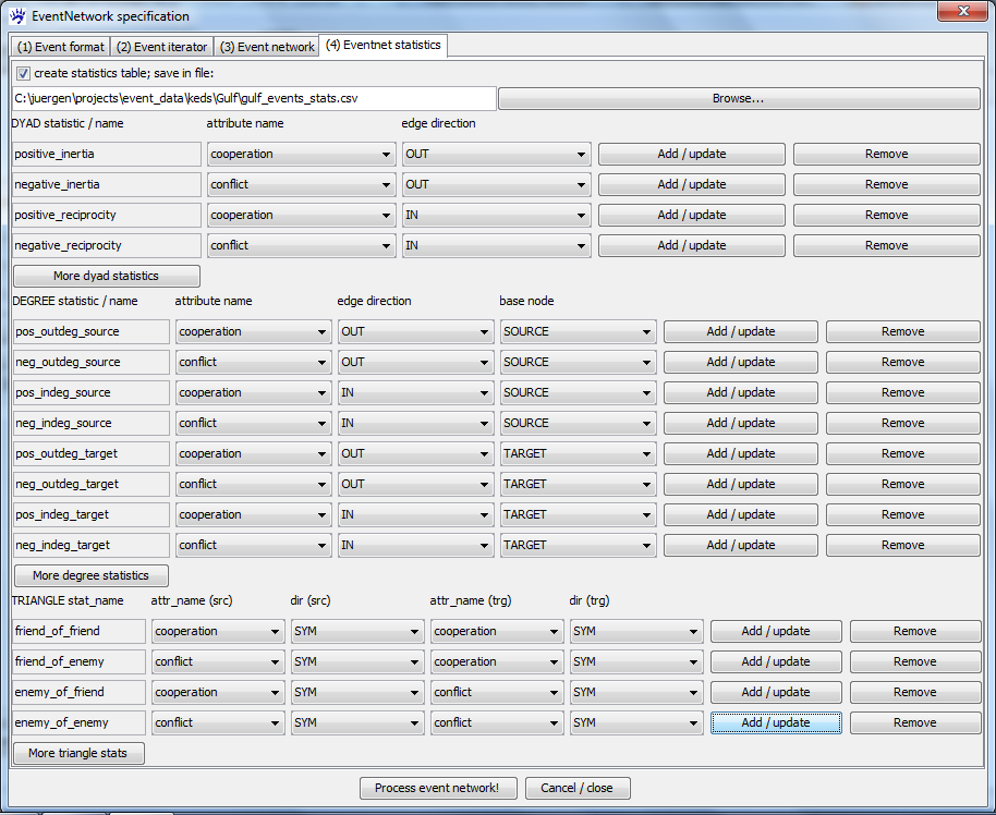
The statistics to be computed are defined in the eventnet statistics tab of the import dialog (see below). You first have to specify whether a statistic table should be created at all; if yes an output file has to be chosen and one or more statistics have to be defined.

The statistics are used to model events in the following way: whenever an event happens that is initiated by a source node and directed to a target node, then the dyad (source, target) is embedded in the network of past events, i.e., all events that happened before the current event. The event network statistics describe relevant aspects of this network of past events with respect to the specific dyad. visone offers three different types of statistics - dyad statistics, degree statistics, and triangle statistics - that can be varied with respect to edge direction and/or link attributes. After defining the statistics they have to be added to the event network by clicking on the Add / update button.

Dyad statistics

Dyad statistics encode aspects of the past events from source to target or in the other direction. That is the dyad statistics encode how source interacted with target in the past or how target interacted with source. In our exmple we define four different dyad statistics that are obtained by switching the direction (inertia if OUT-going events - from source to target - are considered and reciprocity if IN-coming events - from target to source - are considered) and the link attribute (positive for past cooperation and negative for past conflict).

Intuitively, if actors tend to retalliate, then we expect that the negative reciprocity statistic is negatively related with the weight of the next event.

Degree statistics

Degree statistics summarize the past events around the dyad (source, target) by the weighted (out-/in-) degree of source or target. The links can be weighted by any attribute. For instance, the neg_outdeg_source statistic adds up the values of the conflict attribute on all links starting at the source node (not only those that are directed to target).

Intuitively, if actors that initiated a lot of conflictive events in the past tend to do so in the future, then we expect a negative relation between the neg_outdeg_source statistic and the weight of events.

Triangle statistics

Triangle statistics summarize the network of past events around the dyad (source, target) by typed and weighted indirect relations from source over any third node to target or the other way round. You can select the attributes for the links attached to source and to target and the direction which can be OUT (only out-going ties with respect to source/target), IN (only in-coming ties), or SYM (adding up the attributes of out-going and in-coming ties).

For instance, the statistic enemy_of_friend iterates over all actors A in the network, multiplies the value of the cooperation attribute on links connecting source and A (in both directions) with the value of the conflict attribute on links connecting target and A (in both directions), adds up these products for all A, and returns the square root of this sum. Intuitively, the value of the enemy_of_friend statistic on the dyad (source, target) is high if there are many other actors A that cooperated with source and were in conflict with target; structural balance theory predicts that source is then more likely to fight target.

Starting the computation

Once the output file and the statistics are specified, click on the Process event network! button. Snapshots are created as defined in the event iterator tab and statistics are computed as defined in the eventnet statistics tab.

Note that statistics associated with an event that happens at time t are only a function of events that happend earlier (strictly before t) - and do not depend on events that happen in the same time unit.

The computed eventnet statistics file (gulf_events_stats.csv in our example) is a table in CSV format in which each row corresponds to one event of the input file. The components of the event (source, target, time, type, and weight) are first repeated - followed by the values of all statistics.

Computing the statistics for all 300,000 events may take some five to ten minutes on a current standard laptop. Once the computation is finished you see the message processing successfull in the eventnet dialog. If you get an error message you might have a look at the visone console where you can get more information.

Modeling the conditional event weight

The statistics file can now be analyzed with any statistical software - we describe the following for the R environment for statistical computing (also see the visone tutorial on the R console).

First set the R working directory to the directory where the statistics file is located, for instance

 setwd("c:/juergen/projects/event_data/keds/Gulf/")

To read the file into a table and see some summary statistics type

 eventnet.stats <- read.csv("gulf_events_stats.csv", sep=";")
 summary(eventnet.stats)

We model only those events that are not self-loops (loops could have been removed already while preprocessing the input event list - these two procedures are not equivalent since in our case statistics are also functions of loops).

 eventnet.stats <- eventnet.stats[as.character(eventnet.stats$SOURCE) != as.character(eventnet.stats$TARGET),]
 summary(eventnet.stats)

A first very simple model is a linear model for the event weigth (from source to target) - explained by the past conflictive events in the other direction (that is from target directed to the source node).

 model.1 <- lm(WEIGHT ~ 1 + negative_reciprocity, data = eventnet.stats)
 summary(model.1)

A summary of the estimated model yields (among others) the following output:

 Coefficients:
                        Estimate Std. Error t value Pr(>|t|)    
 (Intercept)          -5.730e-01  8.866e-03  -64.63   <2e-16 ***
 negative_reciprocity -2.629e-03  2.829e-05  -92.92   <2e-16 ***
 ---
 Signif. codes:  0 ‘***’ 0.001 ‘**’ 0.01 ‘*’ 0.05 ‘.’ 0.1 ‘ ’ 1

The interpretation is that there seems to be a habit of retalliation: if target has initiated conflictive events towards source then the weight of events from source to target has a tendency to be smaller (significantly negative coefficient for the negative_reciprocity statistic) meaning that the event type is drawn towards conflict. The value of the coefficient (about -0.003) seems to be very small. However this parameter summarizes the change in the event weight when negative_reciprocity increases by one. Typing

 sd(eventnet.stats$negative_reciprocity)

we see that the standard deviation of this statistic is around 290 - meaning that the negative_reciprocity indicator typically varies in the hundreds.

A more complex model tests for structural balance effects, controlling for variation in degrees and direct past interaction. (This is the model taken from Brandes et al.(2009).)

 model.2 <- lm(WEIGHT ~ 1 + positive_inertia + negative_inertia + 
                        positive_reciprocity + negative_reciprocity + 
                        pos_outdeg_source + neg_outdeg_source + 
                        pos_indeg_source + neg_indeg_source + 
                        pos_outdeg_target + neg_outdeg_target + 
                        pos_indeg_target + neg_indeg_target +
                        friend_of_friend + friend_of_enemy + 
                        enemy_of_friend + enemy_of_enemy, 
               data = eventnet.stats)

We get the following results.

 Coefficients:
                        Estimate Std. Error t value Pr(>|t|)    
 (Intercept)          -7.707e-01  1.127e-02 -68.371  < 2e-16 ***
 positive_inertia      5.814e-03  2.723e-04  21.347  < 2e-16 ***
 negative_inertia     -2.145e-03  7.214e-05 -29.730  < 2e-16 ***
 positive_reciprocity  3.071e-03  3.125e-04   9.827  < 2e-16 ***
 negative_reciprocity -2.188e-03  8.175e-05 -26.768  < 2e-16 ***
 pos_outdeg_source     1.391e-03  6.853e-05  20.295  < 2e-16 ***
 neg_outdeg_source    -2.426e-04  3.250e-05  -7.463 8.48e-14 ***
 pos_indeg_source     -6.058e-04  1.022e-04  -5.930 3.02e-09 ***
 neg_indeg_source      1.028e-04  3.259e-05   3.153 0.001615 ** 
 pos_outdeg_target     9.800e-04  7.372e-05  13.293  < 2e-16 ***
 neg_outdeg_target     2.142e-05  3.192e-05   0.671 0.502180    
 pos_indeg_target     -6.572e-04  9.495e-05  -6.922 4.48e-12 ***
 neg_indeg_target      6.988e-05  3.051e-05   2.290 0.022014 *  
 friend_of_friend      1.884e-03  5.349e-04   3.523 0.000427 ***
 friend_of_enemy      -8.913e-04  2.912e-04  -3.061 0.002205 ** 
 enemy_of_friend      -1.308e-03  2.874e-04  -4.553 5.30e-06 ***
 enemy_of_enemy       -1.935e-04  1.532e-04  -1.263 0.206593    
 ---
 Signif. codes:  0 ‘***’ 0.001 ‘**’ 0.01 ‘*’ 0.05 ‘.’ 0.1 ‘ ’ 1

Among other results, this model provides evidence for some - but not all - hypotheses derived from structural balance theory: friends of friends tend to interact more cooperatively while friend of enemies as well as enemies of friends have a tendency to fight each other. On the other hand, the parameter associated with the enemy_of_enemy statistic is not significant. Note that the data set for fitting this model is different from the one taken in Brandes et al. (2009) since here we also included self-loops to compute the statistics (although events connecting an actor with itself have not been used when fitting the linear model).

Obviously, modeling the event type or event weight as a stochastic function of the event network statistics is not restricted to linear models. Furthermore, if the model should control for actor-level or dyad-level covariates (such as the population size of a country or an indicator for whether two countries have a common border), these can be merged into the statistics table after processing of the event network.

References

Carter T. Butts: A Relational event framework for social action. Sociological Methodology 38(1):155-200, 2008.
Ulrik Brandes, Jürgen Lerner, and Tom A. B. Snijders: Networks Evolving Step by Step: Statistical Analysis of Dyadic Event Data. Proc. 2009 Intl. Conf. Advances in Social Network Analysis and Mining (ASONAM 2009), pp.200-205. IEEE Computer Society, 2009.

Event networks (tutorial)

Contents

Example data: networks of political conflict and cooperation

Importing event networks

Event format

Event iterator

Event network

Visualization and analysis of event networks

Statistical modeling of the conditional event type or weight

Event statistics

Dyad statistics

Degree statistics

Triangle statistics

Starting the computation

Modeling the conditional event weight

References

Navigation menu

Event networks (tutorial)

Example data: networks of political conflict and cooperation

Importing event networks

Event format

Event iterator

Event network

Visualization and analysis of event networks

Statistical modeling of the conditional event type or weight

Event statistics

Dyad statistics

Degree statistics

Triangle statistics

Starting the computation

Modeling the conditional event weight

References

Navigation menu

Search