Managing attributes (tutorial): Difference between revisions
| (2 intermediate revisions by the same user not shown) | |||
| Line 12: | Line 12: | ||
== Import the CSV files == | == Import the CSV files == | ||
We start by importing one of the adjacency matrices (e.g., ''newfrat01.csv'') into visone. Therefore use the menu '''file, open''' and select '''files of type''' '' | We start by importing one of the adjacency matrices (e.g., ''newfrat01.csv'') into visone. Therefore use the menu '''file, open''' and select '''files of type''' ''CSV files (.txt, .csv)''. The image below shows the [[import options dialog]] which opens next. We can choose between different data formats in the top most drop-down menu. Since we want to import an adjacency matrix we have to select '''adjacency matrix''' as data format. | ||
[[File:Import_options_newfrat.png]] | [[File:Import_options_newfrat.png]] | ||
[[File:Newfrat01.png|100px|thumb|right]] Setting the options as shown above and clicking on '''ok''' opens the network which looks like the one shown on the right. | [[File:Newfrat01.png|100px|thumb|right]] Setting the other options as shown above and clicking on '''ok''' opens the network which looks like the one shown on the right. | ||
It can be seen that the network is complete (i.e., each pair of actors is connected by a bidirectional tie. All links have an attribute called '''csv value''' whose value corresponds to the respective entry in the adjacency matrix and, thus, is equal to the '''rank''' of the target node in the ordered list of friends of the source node. | It can be seen that the network is complete (i.e., each pair of actors is connected by a bidirectional tie. All links have an attribute called '''csv value''' whose value corresponds to the respective entry in the adjacency matrix and, thus, is equal to the '''rank''' of the target node in the ordered list of friends of the source node. | ||
| Line 36: | Line 36: | ||
[[File:Attribute_manager_filter_rank.png]] | [[File:Attribute_manager_filter_rank.png]] | ||
[[File:Newfrat01_top3.png|100px|thumb|right]] This should select 221 out of 272 links (this information can be found in the lower left corner of the visone window) that can now be deleted by clicking on the menu '''links, delete links''', or from the [[link context menu]]. Clicking on the [[Quick_layout|quick layout button]] should show a network like the one on the right. | [[File:Newfrat01_top3.png|100px|thumb|right]] This should select 221 out of 272 links (this information can be found in the lower left corner of the visone window) that can now be deleted by clicking on the menu '''links, delete links''', or from the [[link context menu]]. Clicking on the [[Quick_layout|quick layout button]] should show a network like the one on the right. If the attribute '''id''' is visualized as node label (via [[Visualization and analysis (tutorial)#Mapping attributes to graphics: categorical attributes|mapping its value]]) it can be seen from this image that nodes 16 and 10 seem to be quite popular. | ||
== Status layouts == | == Status layouts == | ||
| Line 42: | Line 42: | ||
To state this more quantitiatively, we compute the nodes' '''indegree''' via the [[analysis tab]] (ignoring the tie weights by selecting '''link strength'''=''uniform'') and save it in an attribute ''indegree (unweighted)''. This node attribute encodes, thus, the number of times that the node has been nominated as best friend, 2nd best friend, or 3rd best friend. | To state this more quantitiatively, we compute the nodes' '''indegree''' via the [[analysis tab]] (ignoring the tie weights by selecting '''link strength'''=''uniform'') and save it in an attribute ''indegree (unweighted)''. This node attribute encodes, thus, the number of times that the node has been nominated as best friend, 2nd best friend, or 3rd best friend. | ||
[[File:Analysis_tab_indegree.png| | [[File:Analysis_tab_indegree.png|x425px]] [[File:Visualization_tab_status.png|500px]] | ||
To visualize the relative values we use a [[status layout]] that can be computed via the [[visualization tab]] (set '''node value''' to the newly computed node attribute ''indegree (unweighted)'' as shown in the screen shot above). | To visualize the relative values we use a [[status layout]] that can be computed via the [[visualization tab]] (set '''node value''' to the newly computed node attribute ''indegree (unweighted)'' as shown in the screen shot above). | ||
Latest revision as of 09:28, 7 May 2015
This tutorial introduces you to the full power of visone's attribute manager and shows you how to select elements dependent on attribute values. The attribute manager allows you, for instance, to convert tie strength to distance or rankings and vice versa, dichotomize networks, rescale tie weights and much more.
This tutorial assumes that you have a basic understanding of how to analyze and visualize networks in visone - as it is illustrated, for instance, in the previous tutorial.
An exemplary dataset: Newcomb Fraternity Data
The Newcomb Fraternity Data (see Newcomb T. (1961). The acquaintance process. New York: Holt, Reinhard & Winston.) consits of 15 matrices recording weekly sociometric preference rankings from 17 men attending the University of Michigan in the fall of 1956. Each participant ranks all 16 others from best friend down to least friend. This data set is explained in more detail on the page Newcomb Fraternity (data).
To follow the steps illustrated in this tutorial, you should download the file Newfrat.zip (ZIP file containing the 15 matrices newfrat01.csv to newfrat15.csv), save it to your computer and decompress (unzip) it.
Import the CSV files
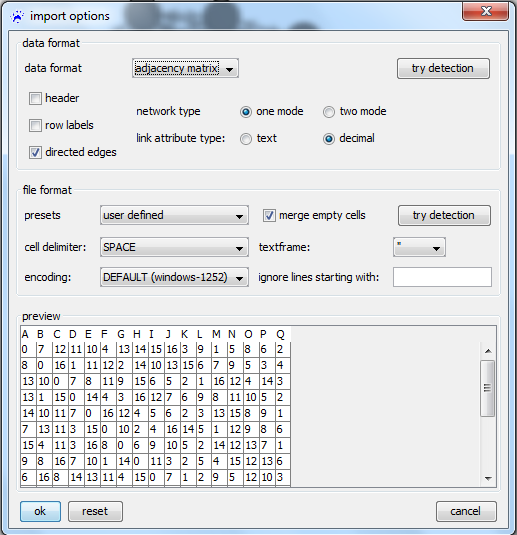
We start by importing one of the adjacency matrices (e.g., newfrat01.csv) into visone. Therefore use the menu file, open and select files of type CSV files (.txt, .csv). The image below shows the import options dialog which opens next. We can choose between different data formats in the top most drop-down menu. Since we want to import an adjacency matrix we have to select adjacency matrix as data format.
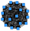
Setting the other options as shown above and clicking on ok opens the network which looks like the one shown on the right.
It can be seen that the network is complete (i.e., each pair of actors is connected by a bidirectional tie. All links have an attribute called csv value whose value corresponds to the respective entry in the adjacency matrix and, thus, is equal to the rank of the target node in the ordered list of friends of the source node.
A more exhaustive treatment of how to import data into visone is given in the data input tutorial.
Who is the most popular?
For illustration, we want to explore the popularity of actors with respect to the aggregated nominations of all others. Clearly, the number of incomming ties would not be a good measure for this, since each node receives exactly 16 links. The information about how popular actors are lies in the ranking of the ties. In the extremal case it would be possible that one actor (the most popular one) receives 16 links having rank equal to 1 and another actor receives 16 links labeled 16 (i.e., this actor would be the least friend for all others).
There are several possibilities to turn the weighted nominations into a one-dimensional measure for popularity: dichotomizing the network by defining a threshold that separates between the "friends" and the "non-friends"; computing a weighted indegree that takes into account the link weights; or combinations of the two. Some of these possibilities are illustrated below.
Selecting and deleting links below a threshold
It is convenient to rename the attribute encoding the ranks, since csv value is not a very intuitive name. To do this open the attribute manager, click the button link in the top row, and configure on the left. Click in the text field where it currently says csv value and write, for instance, rank into it; click on the apply button.
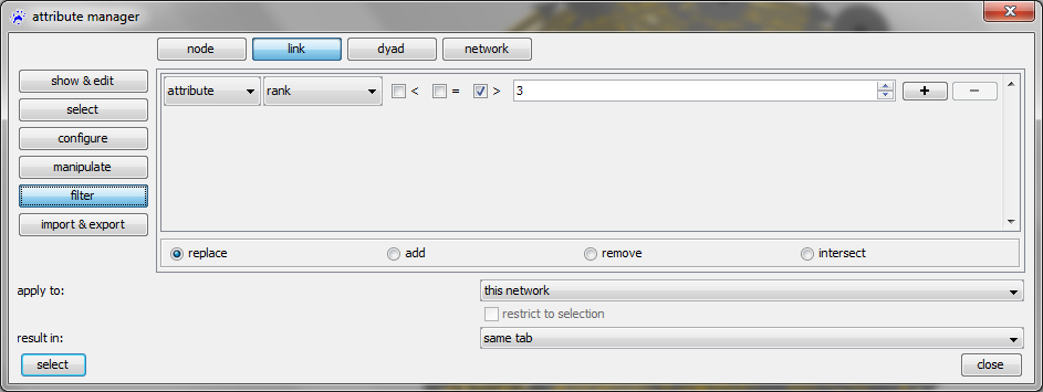
Exemplarily, we want to keep only links that go to the top-3 friends. To select all links with a rank higher than 3 (i.e., all links that we want to delete) click on the button filter on the left-hand side (still having selected link in the top row). In the row where you can define the filter, select attribute, then rank, check (only) the box before the greater than-sign (>), type 3 in the textfield. Select the radio button replace at the bottom and click on select
This should select 221 out of 272 links (this information can be found in the lower left corner of the visone window) that can now be deleted by clicking on the menu links, delete links, or from the link context menu. Clicking on the quick layout button should show a network like the one on the right. If the attribute id is visualized as node label (via mapping its value) it can be seen from this image that nodes 16 and 10 seem to be quite popular.
Status layouts
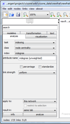
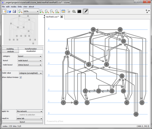
To state this more quantitiatively, we compute the nodes' indegree via the analysis tab (ignoring the tie weights by selecting link strength=uniform) and save it in an attribute indegree (unweighted). This node attribute encodes, thus, the number of times that the node has been nominated as best friend, 2nd best friend, or 3rd best friend.
To visualize the relative values we use a status layout that can be computed via the visualization tab (set node value to the newly computed node attribute indegree (unweighted) as shown in the screen shot above).
Transforming attributes
The unweighted indegree as computed above counts the number of times that the node has been nominated as 1st, 2nd, or 3rd best friend. To count nominations as best friend more than nominations as 2nd best friend, we can map these rankings to values and then compute the weighted indegrees. The rank values can not directly be taken as measures of tie strength since a higher rank (e.g., 3) indicates a lower friendship intensity than a lower rank (e.g., 1). Thus we have to apply an order-reversing mapping on the rank attribute. This can be done via the attribute manager. Note that the particular choice for the transformation below has been done arbitrarily and merely serves for illustrating how attributes can be transformed; when a particular research questions has to be answered one should be able to justify such a choice, or show that the particular choice of transformation does not influence the findings significantly.
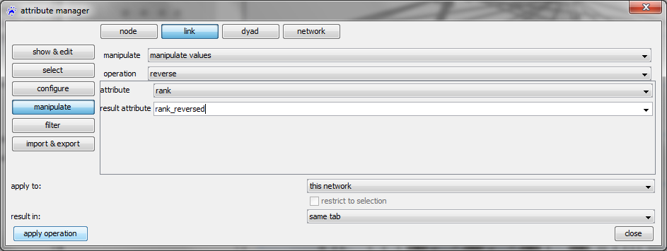
In the attribute manager select the link button on the top and manipulate on the left. Selecting, from top to bottom, manipulate values, reverse, and rank, giving a new name to the transformed attribute (such as rank reversed), and clicking the apply button adds the new attribute to all nodes. Reverse means that the interval of values gets reverted as specified by the formula
.
In our example, 1 is mapped to 3, 2 to 2, and 3 to 1. You might inspect the other possibilities for transforming attribute values; note that transformations that are not directly implemented in the attribute manager can be done via visone's R console (see the R console tutorial for illustration).
Centrality and status on weighted networks
A weighted indegree, dependent on the newly computed attribute, can be computed via the analysis tab (similar to the unweighted indegree, but setting link strength to rank reversed). Mapping this weighted indegree in a status layout reveals that actor 16 is more popular than 10 with respect to the weighted measure, but equally popular with respect to the unweighted indegree.
