Personal networks (tutorial): Difference between revisions
No edit summary |
|||
| (14 intermediate revisions by the same user not shown) | |||
| Line 1: | Line 1: | ||
[http://sourceforge.net/projects/egonet/ EgoNet] is a software to conduct interviews in which the [[Personal_network|personal networks]] of respondents are collected. This tutorial explains (1) how to load data collected with EgoNet into visone and (2) how to cluster, aggregate, and visualize collections of personal networks using the methodology proposed in: Ulrik Brandes, Juergen Lerner, Miranda J. Lubbers, Chris McCarty, and Jose Luis Molina '''"Visual Statistics for Collections of Clustered Graphs"'''. ''Proc. IEEE Pacific Visualization Symp. (PacificVis'08)'', 2008 ([http://www.inf.uni-konstanz.de/algo/publications/bllmm-vsccg-08.pdf ''link to pdf'']). | [http://sourceforge.net/projects/egonet/ EgoNet] is a software to conduct interviews in which the [[Personal_network|personal networks]] of respondents are collected. This [[Tutorials|tutorial]] explains (1) how to load data collected with EgoNet into visone and (2) how to cluster, aggregate, and visualize collections of personal networks using the methodology proposed in: Ulrik Brandes, Juergen Lerner, Miranda J. Lubbers, Chris McCarty, and Jose Luis Molina '''"Visual Statistics for Collections of Clustered Graphs"'''. ''Proc. IEEE Pacific Visualization Symp. (PacificVis'08)'', 2008 ([http://www.inf.uni-konstanz.de/algo/publications/bllmm-vsccg-08.pdf ''link to pdf'']). | ||
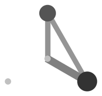
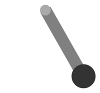
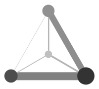
For instance, the three images below (from left to right) represent the ''median class-level network'' of Chinese, Filipino, and Sikh immigrants in Barcelona. | |||
[[File:Average_clustered_chinese.png|200px]] [[File:Average_clustered_filipino.png|200px]] [[File:Average_clustered_sikh.png|200px]] [[File:Chinese_clustered_labeled.png|200px]] | |||
To follow the steps outlined in this tutorial you should download the [[Signos_(data)|'''Signos data''']] and extract (unzip) the file on your computer. Furthermore you need the [[EgoNet2GraphML_(software)|'''EgoNet2GraphML''' software]] to convert EgoNet interviews to GraphML files and apply the clustering and aggregation. | To follow the steps outlined in this tutorial you should download the [[Signos_(data)|'''Signos data''']] and extract (unzip) the file on your computer. Furthermore you need the [[EgoNet2GraphML_(software)|'''EgoNet2GraphML''' software]] to convert EgoNet interviews to GraphML files and apply the clustering and aggregation. | ||
== Converting EgoNet interviews | Please address questions and comments about this tutorial to me ([[User:Lerner|Jürgen Lerner]]). | ||
== Converting EgoNet interviews to GraphML files == | |||
To open EgoNet interviews with visone you first have to convert these to [[GraphML]] with the [[EgoNet2GraphML_(software)|EgoNet2GraphML software]]. When you have downloaded the file '''EgoNet2GraphML.jar''' from the [http://www.inf.uni-konstanz.de/algo/software/egonet2graphml/ EgoNet2GraphML website] execute it (for instance by double-clicking). The main window opens as shown below. | To open EgoNet interviews with visone you first have to convert these to [[GraphML]] with the [[EgoNet2GraphML_(software)|EgoNet2GraphML software]]. When you have downloaded the file '''EgoNet2GraphML.jar''' from the [http://www.inf.uni-konstanz.de/algo/software/egonet2graphml/ EgoNet2GraphML website] execute it (for instance by double-clicking). The main window opens as shown below. | ||
| Line 121: | Line 127: | ||
* To set the coordinates map the attribute '''X-coord''' to the x axis and '''Y-coord''' to the y axis. To do this go to the [[visualization tab]], chose '''category'''=''mapping'', '''type'''=''coordinates'', '''property'''=''cartesian'', '''attribute'''=''X-coord'' (respectively ''Y-coord''), and '''map to'''=''x axis'' (respectively ''y axis''). Think of selecting '''apply to'''=''open networks'' and click the '''visualize!''' button. | * To set the coordinates map the attribute '''X-coord''' to the x axis and '''Y-coord''' to the y axis. To do this go to the [[visualization tab]], chose '''category'''=''mapping'', '''type'''=''coordinates'', '''property'''=''cartesian'', '''attribute'''=''X-coord'' (respectively ''Y-coord''), and '''map to'''=''x axis'' (respectively ''y axis''). Think of selecting '''apply to'''=''open networks'' and click the '''visualize!''' button. | ||
* If you want to show the labels (which is appropriate to show which node represents which class) you can also map the attribute ''class label'' to the node label. | * If you want to show the labels (which is appropriate to show which node represents which class) you can also map the attribute ''class label'' to the node label. | ||
* To represent the class size chose '''type'''=''size'' and '''property'''=''node area''. In our example it does not matter whether you take the attribute ''class size'' or ''relative class size'' since these are a constant factor of each other. Alternatively you could map class size to the class label (if you want to include these in the images). | * To represent the class size chose '''type'''=''size'' and '''property'''=''node area''. In our example it does not matter whether you take the attribute ''class size'' or ''relative class size'' since these are a constant factor of each other. Alternatively you could map class size to the class label (if you want to include these in the images). | ||
* The intra-class tie weight can be represented by a color gradient of the node color. To do this chose '''type'''=''color'', '''property'''=''node color'', '''method'''=''interpolation''. Then decide on a color that represents the maximum value (the strongest intra-class connectivity) and one for the minimum value. A choice that always works well is, for instance, dark gray and light gray; but red and blue or any other choice would be possible. | |||
* Similarly the inter-class tie weight can be mapped to the link color and/or to the link width. | |||
Altogether it should be possible to create images like the following. | |||
[[File:Chinese0_clustered.png|100px]] | |||
[[File:Chinese1_clustered.png|100px]] | |||
[[File:Chinese2_clustered.png|100px]] | |||
[[File:Chinese3_clustered.png|100px]] | |||
[[File:Chinese4_clustered.png|100px]] | |||
[[File:Chinese5_clustered.png|100px]] | |||
[[File:Chinese6_clustered.png|100px]] | |||
[[File:Chinese7_clustered.png|100px]] | |||
[[File:Chinese8_clustered.png|100px]] | |||
[[File:Chinese9_clustered.png|100px]] | |||
[[File:Chinese10_clustered.png|100px]] | |||
[[File:Chinese11_clustered.png|100px]] | |||
[[File:Chinese12_clustered.png|100px]] | |||
[[File:Chinese13_clustered.png|100px]] | |||
[[File:Chinese14_clustered.png|100px]] | |||
[[File:Chinese15_clustered.png|100px]] | |||
[[File:Chinese16_clustered.png|100px]] | |||
[[File:Chinese17_clustered.png|100px]] | |||
[[File:Chinese18_clustered.png|100px]] | |||
[[File:Chinese19_clustered.png|100px]] | |||
[[File:Chinese20_clustered.png|100px]] | |||
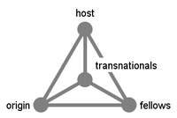
Drawing such class-level networks side by side allows simple and fast comparison and to spot networks where certain classes are particularly large or small or densely or weakly connected. We propose '''not''' to draw node labels in such collections of network images but rather show the labels (and thus the stable positions of the classes) only once (see below). | |||
[[File:Chinese_clustered_labeled.png|250px]] | |||
Some comments might be helpful. | |||
* To save the images in image files use the menu '''file''', '''export''' and select an approriate image format. (We recommend PDF for printing or use in [http://en.wikipedia.org/wiki/LaTeX LaTeX] documents; for webpages you could, e.g., use PNG as we did here in this tutorial.) | |||
* visone has a minimum node size and link width. To hide the classes of size zero and the links with weight zero you have to either delete these or (preferable) to color them with ''no color'' in the [[node properties dialog]]. (The latter version is preferable since then you get the same bounding box when exporting the images.) | |||
* If the average node size (or link width) is too small or too large, you can increase or decrease the size of all nodes (respectively, width of all links) before mapping class size or tie weight to them. This can be done "by hand" with the [[node properties dialog]] or you define an appropriate [[Node_templates_dialog|node template]] (respectively [[Link_templates_dialog|link template]]) before opening the GraphML files. | |||
* When mapping attributes to a color gradient visone does (currently) not offer you to take the maximum/minimum values over the whole collection. Thus the darkest/brightest color has a different meaning in the different networks. This will be improved in future versions of visone. | |||
You might find other ways to visually represent class-level networks with the given indicators. Of course, the attributes of class-level networks can also be send via visone's [[Console|R console]] to the [http://www.r-project.org/ R software for statistical computing], or they can be exported to attribute tables via the [[attribute manager]], thereby allowing external analysis of the networks' characteristics. | |||
== Tendency and dispersion in collections of personal networks == | == Tendency and dispersion in collections of personal networks == | ||
It is often insightful to look at the "average" personal networks of respondents from various communities. In the given example, a typical questions would be whether Chinese immigrants have a systematically different network than the Filipins or Sikhs. When clustering a collection of personal networks (as we did above) EgoNet2GraphML generates one additional network file named <code>Average_clustered.graphml</code>. This average network has the same classes as the individual class-level networks; its node and link attributes are componentwise averages over the attributes of the individual networks. We compute and store several measures for central tendency and dispersion of the various indicators. See below the node and link attributes of the average class level network over the 21 networks of Chinese respondents. | |||
[[File:EgoNet2GraphML_average_attributes.png]] | |||
[[File:EgoNet2GraphML_average_link_attributes.png]] | |||
In detail, for each of the measures ''relative class size'', ''intra-class weight'', and ''inter-class weight'' of the individual networks, we obtain as measures of central tendency the '''mean''' and '''median''' over the community and as measures of dispersion the '''standard deviation''', '''1st quartile''', and '''3rd quartile'''. | |||
The following three images show (from left to right) the median values for the Chinese, Filipino, and Sikh community (the rightmost images recalls the positions of the classes). | |||
[[File:Average_clustered_chinese.png|200px]] [[File:Average_clustered_filipino.png|200px]] [[File:Average_clustered_sikh.png|200px]] [[File:Chinese_clustered_labeled.png|200px]] | |||
It can be seen that the "typical" (meaning median) Chinese immigrant knows many ''fellow'' migrants (from China to Spain) and members from the ''host'' class (Spanish); the ''origin'' class (Chinese alters still living in China) is relatively small and not well connected to the other classes (for at least half of the migrants). The median network of the Filipinos is even more focussed on the ''fellows'' and ''host'' class. The median network of the Sikhs is more balanced: there the largest class is again composed of ''fellow'' migrants; ''origin'' and ''host'' are not so much smaller but the ''host'' class is sparser connected (less intra-class ties) than the ''origin'' class. | |||
Latest revision as of 08:37, 19 March 2014
EgoNet is a software to conduct interviews in which the personal networks of respondents are collected. This tutorial explains (1) how to load data collected with EgoNet into visone and (2) how to cluster, aggregate, and visualize collections of personal networks using the methodology proposed in: Ulrik Brandes, Juergen Lerner, Miranda J. Lubbers, Chris McCarty, and Jose Luis Molina "Visual Statistics for Collections of Clustered Graphs". Proc. IEEE Pacific Visualization Symp. (PacificVis'08), 2008 (link to pdf).
For instance, the three images below (from left to right) represent the median class-level network of Chinese, Filipino, and Sikh immigrants in Barcelona.
To follow the steps outlined in this tutorial you should download the Signos data and extract (unzip) the file on your computer. Furthermore you need the EgoNet2GraphML software to convert EgoNet interviews to GraphML files and apply the clustering and aggregation.
Please address questions and comments about this tutorial to me (Jürgen Lerner).
Converting EgoNet interviews to GraphML files
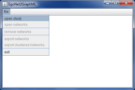
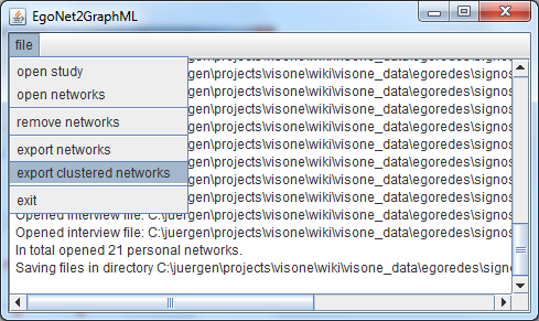
To open EgoNet interviews with visone you first have to convert these to GraphML with the EgoNet2GraphML software. When you have downloaded the file EgoNet2GraphML.jar from the EgoNet2GraphML website execute it (for instance by double-clicking). The main window opens as shown below.
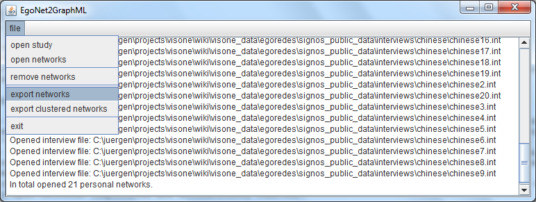
To convert EgoNet interviews to GraphML you first have to open a study definition file (filename extension .ego) and then one or more interview files (filename extension .int) that have been collected with the selected study definition file. Click on the open study menu item, select the file signos.ego in the previously downloaded signos_public_data (see above) and click on the open button. Then click on the open networks menu item, navigate to the directory interviews/chinese (for instance) and select the interview files to open. You may add the files one by one, or select several of them at once (by keeping the Control-key down while selecting), or select all .int files in the current directory by typing Control-A. You get short messages about each file you opened as well as the total number of currently open networks (duplicates are automatically removed).
To convert the interview files to GraphML click on the export networks menu item, select a directory to save the files (you might, for instance, create a new directory graphml as a subfolder of the chinese directory), and click the Export! button. EgoNet2GraphML exports all currently open networks to GraphML files; the filenames are the ones of the interview files - just with the extension .int replaced by .graphml.
The GraphML files can be opened, analyzed, and visualized with visone (not with EgoNet2GraphML) as explained in the following. The networks have a node for each alter and store the questions about ego as network-level attributes and the questions about alters as node attributes. Typically, the respondent has to evaluate the relation between every undirected pair of alters; in this case the resulting network is complete and the alter-alter responses are encoded as link attributes.
Visual analysis of personal networks on the individual level
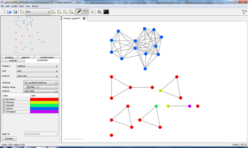
Visual analysis of the networks on the individual level is similar to the one presented in the tutorial on visualization and analysis which you might consult as well. When opening one of the newly generated GraphML files (for instance, chinese1.graphml) with visone you see (in the lower left corner) that the network has 30 nodes and 435 links (it is a complete network). Most of the information is actually contained in node attributes, link attributes, and network attributes. Open the attribute manager to see what is there.
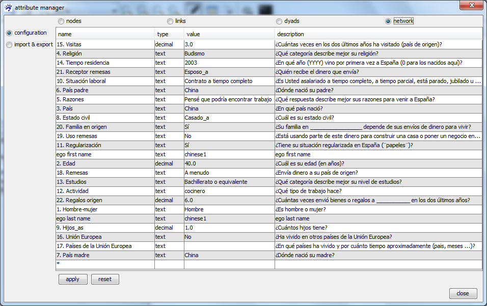
The questions (and answers) about ego are available as network attributes (see the image below). The name of the attribute is the title of the question, the attribute description gives the exact formulation of the question. The type is text for most attributes; for some (numerical) attributes it is decimal. The values give the responses to the respective question.
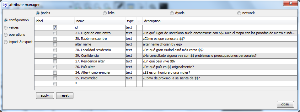
Similarly, the questions about alters are available as node attributes (see below). Note that for node attributes there is a (potentially) different value for each of the 30 alters (which can be shown by selecting the values radio button on the left-hand side of the attribute manager).
Similarly, the questions about the alter-alter pairs are available as link attributes (see below). Here we have a (potentially) different value for each of the 435 pairs of alters.
A typical approach to visually explore such a personal network is the following:
- define which actors are connected by a link, dependent on responses to the alter-alter questions;
- apply a network layout algorithm to reveal the structure of the network;
- map attributes of interest to graphical variables.
Exemplarily we illustrate these steps in the following.
To define which actors are connected by a link we actually have to decide which links we want to delete (because currently every pair of actors is connected). To do so we open visone's selection tab and choose the attribute Alter alter relacion (link) in the drop-down menu. We can see (also see the image on the right-hand side) that this attribute takes one of three values: Muy probablemente (very likely), No es probable (unlikely), or Podria ser (maybe); the wording of the question was Es probable que estas dos personas se relacionen independientemente de Usted?(Is it likely that these two persons meet each other independent of you?) We want to keep only those links that have been evaluated as very likely; therefore we select the two other values in the selection tab (this selects 373 links out of 435, as you can see in the lower left corner of the visone window). The selected links can be deleted via the links menu. Deleting them and then clicking on the quick layout button ![]() reveals the structure of the network. As this is often the case for personal networks, this network decomposes into densely connected clusters.
reveals the structure of the network. As this is often the case for personal networks, this network decomposes into densely connected clusters.
Mapping attributes to graphical variables can be done via the visualization tab (also see the image below). For instance, mapping the attribute Localidad residencia (city of residence) to color shows that the large cluster on the top is composed of actors living in the same (Chinese) city Suzhou; the others live in Spanish cities, most in Barcelona. You might continue to explore the other attributes.
Class-level analysis of personal networks
Especially when analyzing/visualizing collections of many personal networks, it is often not very informative to look at every individual node in every network. The work of Brandes et al. (2008) proposed to simplify networks by classifying actors dependent on attributes. The resulting class-level networks reveal the size of the various classes and how well are actors connected within classes and in-between classes. This information can be visually represented in a concise way so that dozens or hundreds of networks can be shown on the same page revealing typical networks as well as outliers. In addition, class-level networks can be averaged over (sub-)communities revealing systematic differences (or similarities) with respect to the typical personal network composition and structure.
To do such an analysis we go back to the EgoNet2GraphML converter and chose the export clustered networks option in the file menu. (We assume that you still have several networks open in the converter; for instance, all networks from Chinese respondents.)
When you chose this menu item a dialog is started in which EgoNet2GraphML asks you to specify how actors should be classified.
Specifying a network partition based on node attributes
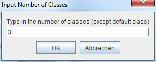
The network partition is specified by the number of classes, the class labels, and a set of rules clarifying which (combinations of) attribute values should be put into which classes. The first dialog box asks for the number of classes (except the default class).
The default class ensures that every alter does fit into one class (if nothing else fits, then the actor is put into the default class). For instance, if you want to define only two classes, say male and female, you type a 1 into the above dialog and subsequently you have to specify one of the classes (say male) and the second class contains all actors that do not fit into the first class. Following the approach of Brandes et al., we want to specify four classes (host, fellows, origin, and transnationals); that's why we type a 3 into the above dialog box and press Enter (or the ok button).
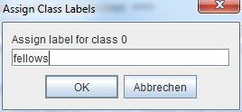
Subsequently we see four dialog boxes asking for the class labels (since class0, class1, ... is not very informative).
We type, for instance, host for class 0, press Enter; then type fellows, press Enter; then origin; and finally transnationals for the default class.
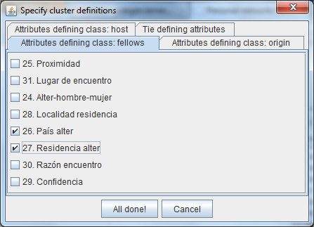
After having set the class labels we see a dialog asking for the definition of each class (except the default class). This dialog has (in our example) four tabs, three for the definition of the classes host, fellows, and origin and one for the attributes defining the ties in the network. Let's turn first to the classes.
The tabs Attributes defining class: ... present a list of all alter attributes. The logic of the class specification is the following.
- when an attribute is not selected (not checked), then this attribute has no impact on whether alters are put into the respective class or not;
- when you select an attribute, then an alter can be in the respective class only if his/her value (of the attribute in question) matches one of several selected possible values;
- finally an alter is in a particular class if he/she satisfies the conditions imposed by all selected attributes.
This becomes clearer when we look at examples.
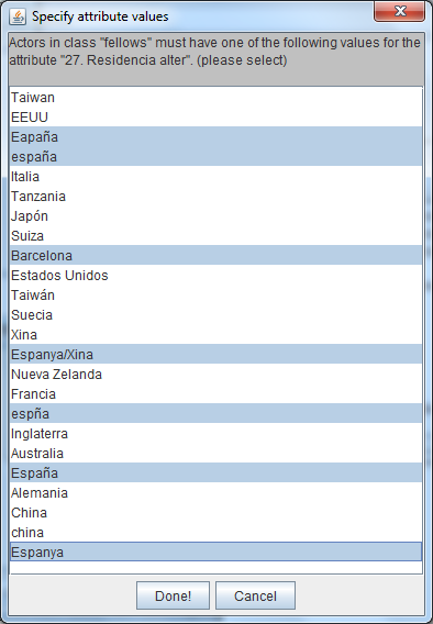
The class fellows contains all migrants stemming from the same country of origin (as ego) and having migrated to the same host country. In our case, if we go to the tab for the fellows class and select the checkbox left of the attribute Residencia alter (meaning country where the actor currently lives), we are presented a list of all values that this attribute takes for any alter in any of the open networks. If we have open all 21 networks from the chinese folder, this list looks like the following.
Since the Chinese respondents (egos) migrated from China to Spain, an alter can be in the fellow class only if his current country of living is Spain. As you can see (above) the respondents have choosen plenty of variants to spell España; select all these variants (keep the Control-key down to select more than one value) and then click on the Done! button. Still in the fellows tab, select the attribute Pais alter (meaning country of origin) and select the values China and china. The specification of the fellows class is now ready; an alter is in this class if his/her Pais alter attribute has the value China or china and his/her Residencia alter attribute has the value España or Espanya or Espña or ...
The class origin consists of alters stemming from the same country of origin as ego and still living there; so in our example this is two times China (or variants thereof). The class host consists of alters stemming from the host country (Spain, also select the value Cataluña). All actors that do not fit in any of these three classes are put into the default class transnationals.
The tab Tie defining attributes works similar. Here we specify which alter-alter pairs are connected by links. In our example we have only one alter-alter attribute Alter alter relacion and select the value Muy probablemente.
Once everything is specified click on the All done! button, select a directory to save the files to (for instance you might create a subfolder graphml_clustered of the chinese directory), and click on Export!.
When the exporting is done, the directory graphml_clustered (or whatever you have choosen) contains 22 GraphML files: the class-level networks obtained from the 21 interviews and one file Average_clustered.graphml which is an aggregation over the whole community of 21 networks. We say more about the average later in this tutorial and first turn to the individual class-level files.
Attributes of class-level networks
The GraphML files can be opened, analyzed, and visualized with visone (not with EgoNet2GraphML). In visone click on open in the file menu and select the 21 files chinese0_clustered.graphml, ..., chinese20_clustered.graphml (not the Average_clustered.graphml) and click on ok. The networks are opened each in its own tab; each has four nodes (corresponding to the four classes) and six links (corresponding to the six undirected pairs of different classes). The information is again contained in node and link attributes; we first describe these attributes and then illustrate how to visualize them.
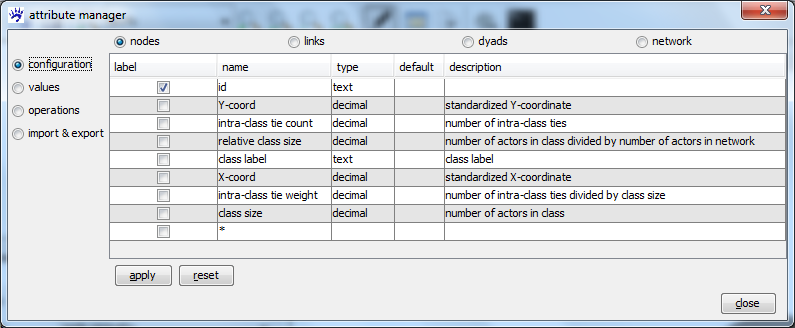
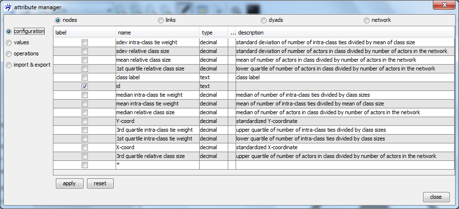
To see the class-level attributes, open the attribute manager ![]() and select nodes and configuration.
and select nodes and configuration.
The attributes fall into different categories:
- class label are the labels that we assigned previously (host, fellows, origin, and transnationals);
- the number of actors in the various classes is given in the attributes class size (unnormalized) and relative class size (normalized); if all networks in the collection have the same number of alters, the two attributes are a constant factor of each other; if networks have different size the relative class size might be more appropriate;
- how well actors in the various classes are connected to each other is given in the attributes intra-class tie count and intra-class tie weight (the latter being the average number of links to members of the same class); normally the weight is more appropriate than the count since it is better comparable across classes of different size (just by chance alone, larger classes are likely to contain more links)
- the attributes X-coord and Y-coord suggest standardized positions for placing the nodes; these values can be taken for a common layout as we will show later;
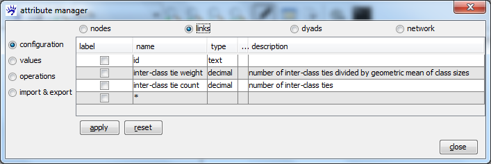
The link attributes are shown by selecting links in the attribute manager.
These attributes encode how well actors in one class are connected to actors in another class. Again we have the unnormalized tie count and the normalized tie weights.
Visual analysis of individual personal networks on the class level
To enable visual comparison between the individual class-level networks we map (some of) their attributes to graphical variables. One possibility to do so is to use the given standardized X-/Y-coordinates to define the positions in the images; to represent class size by the area of the nodes; to represent intra-class tie weight by a color gradient for the node color; and to map the inter-class tie weight to thickness and/or color of the links. In visone these mappings (or others) can be done via the visualization tab; chose category=mapping. An important remark is that you can apply the mappings to all open networks at once. Therefore, before clicking the visualize! button, select apply to=open networks. (It is a necessary condition that the attribute to be mapped is available for all open networks; this is satisfied, for instance, if you have open all 21 class-level networks generated so far and no other network.)
In detail:
- To set the coordinates map the attribute X-coord to the x axis and Y-coord to the y axis. To do this go to the visualization tab, chose category=mapping, type=coordinates, property=cartesian, attribute=X-coord (respectively Y-coord), and map to=x axis (respectively y axis). Think of selecting apply to=open networks and click the visualize! button.
- If you want to show the labels (which is appropriate to show which node represents which class) you can also map the attribute class label to the node label.
- To represent the class size chose type=size and property=node area. In our example it does not matter whether you take the attribute class size or relative class size since these are a constant factor of each other. Alternatively you could map class size to the class label (if you want to include these in the images).
- The intra-class tie weight can be represented by a color gradient of the node color. To do this chose type=color, property=node color, method=interpolation. Then decide on a color that represents the maximum value (the strongest intra-class connectivity) and one for the minimum value. A choice that always works well is, for instance, dark gray and light gray; but red and blue or any other choice would be possible.
- Similarly the inter-class tie weight can be mapped to the link color and/or to the link width.
Altogether it should be possible to create images like the following.
Drawing such class-level networks side by side allows simple and fast comparison and to spot networks where certain classes are particularly large or small or densely or weakly connected. We propose not to draw node labels in such collections of network images but rather show the labels (and thus the stable positions of the classes) only once (see below).
Some comments might be helpful.
- To save the images in image files use the menu file, export and select an approriate image format. (We recommend PDF for printing or use in LaTeX documents; for webpages you could, e.g., use PNG as we did here in this tutorial.)
- visone has a minimum node size and link width. To hide the classes of size zero and the links with weight zero you have to either delete these or (preferable) to color them with no color in the node properties dialog. (The latter version is preferable since then you get the same bounding box when exporting the images.)
- If the average node size (or link width) is too small or too large, you can increase or decrease the size of all nodes (respectively, width of all links) before mapping class size or tie weight to them. This can be done "by hand" with the node properties dialog or you define an appropriate node template (respectively link template) before opening the GraphML files.
- When mapping attributes to a color gradient visone does (currently) not offer you to take the maximum/minimum values over the whole collection. Thus the darkest/brightest color has a different meaning in the different networks. This will be improved in future versions of visone.
You might find other ways to visually represent class-level networks with the given indicators. Of course, the attributes of class-level networks can also be send via visone's R console to the R software for statistical computing, or they can be exported to attribute tables via the attribute manager, thereby allowing external analysis of the networks' characteristics.
Tendency and dispersion in collections of personal networks
It is often insightful to look at the "average" personal networks of respondents from various communities. In the given example, a typical questions would be whether Chinese immigrants have a systematically different network than the Filipins or Sikhs. When clustering a collection of personal networks (as we did above) EgoNet2GraphML generates one additional network file named Average_clustered.graphml. This average network has the same classes as the individual class-level networks; its node and link attributes are componentwise averages over the attributes of the individual networks. We compute and store several measures for central tendency and dispersion of the various indicators. See below the node and link attributes of the average class level network over the 21 networks of Chinese respondents.
In detail, for each of the measures relative class size, intra-class weight, and inter-class weight of the individual networks, we obtain as measures of central tendency the mean and median over the community and as measures of dispersion the standard deviation, 1st quartile, and 3rd quartile.
The following three images show (from left to right) the median values for the Chinese, Filipino, and Sikh community (the rightmost images recalls the positions of the classes).
It can be seen that the "typical" (meaning median) Chinese immigrant knows many fellow migrants (from China to Spain) and members from the host class (Spanish); the origin class (Chinese alters still living in China) is relatively small and not well connected to the other classes (for at least half of the migrants). The median network of the Filipinos is even more focussed on the fellows and host class. The median network of the Sikhs is more balanced: there the largest class is again composed of fellow migrants; origin and host are not so much smaller but the host class is sparser connected (less intra-class ties) than the origin class.
