R console (tutorial)
This tutorial illustrates how to send network data from visone to R and back. The R project for statistical computing offers a rich set of methods for data analysis and modeling which becomes accessible from visone through the R console. We assume that you have installed the R connection as it is explained in the installation tutorial. This tutorial assumes that you have basic understanding about how to work with visone as it is, for instance, explained in the tutorial on visualization and analysis. You do not need to have any previous knowledge about R to follow this tutorial; nevertheless, to exploit the full potential offered by R you could consult documentation and tutorials linked from the R-project page.
To follow the steps illustrated in this tutorial you should download the network file Egonet.graphml which is linked from and explained in the page Egoredes_(data). Further you should remove all ties that are not rated as very likely in the same manner as it is explained in the last section of the visualization and analysis tutorial.
Sending networks from visone to R
You can open the R console by clicking on the ![]() icon in the toolbar.
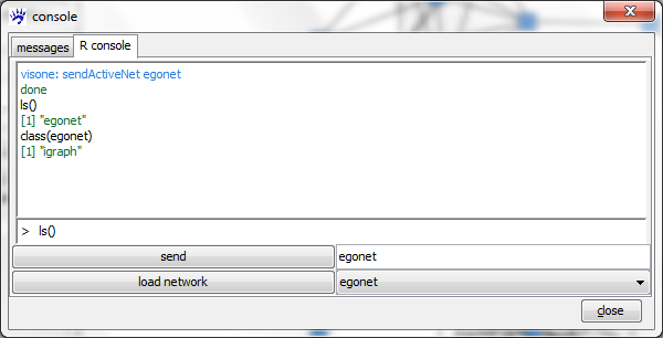
To send the network from visone to R choose a name in the textfield right of the send button (you might just accept visone's suggestion for this name, which should be egonet), and click on the send button. After clicking on send visone starts the Rserve connection and sends the current network to R. If this does not work you should check the settings of the R connection options accessible via the file, options menu. If it works you should get a message like
icon in the toolbar.
To send the network from visone to R choose a name in the textfield right of the send button (you might just accept visone's suggestion for this name, which should be egonet), and click on the send button. After clicking on send visone starts the Rserve connection and sends the current network to R. If this does not work you should check the settings of the R connection options accessible via the file, options menu. If it works you should get a message like
 visone: sendActiveNet egonet
 done
in the message field of the R console.
You can list all variables that are in the R workspace by typing
ls()
in the input field at the bottom of the R console and pressing the Enter-Key (currently there is one object called egonet). Typing
class(egonet)
prints the class of the egonet object which is igraph. igraph is an R package obtainable from the CRAN Website (this site also gives you access to R tutorials and documentation). The igraph package is documented in more detail on http://igraph.sourceforge.net/.
Getting basic statistics about an igraph object
The class of the object egonet in the R workshop is printed when executing the command
class(egonet)
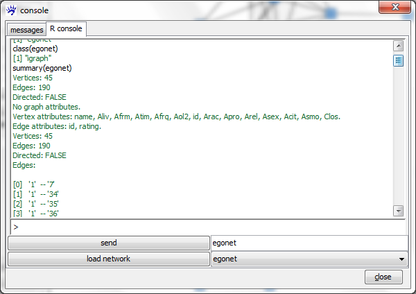
As we can see the class of egonet is igraph. The igraph documentation linked above gives a complete list of all methods available for this class. In the following we describe how to inspect what is encoded in the given object and how to get simple summary statistics. Executing the command
summary(egonet)
outputs basic information such as the number of vertices and edges, the names of vertex and edge attributes, as well as a list of all edges.
Exploring attributes
The names of all vertex or edge attributes are printed with
 list.vertex.attributes(egonet)
 list.edge.attributes(egonet)
To see the values of the vertex or edge attributes one needs to understand the concept of vertex iterators and edge iterators in igraph. The vertex iterator of graph egonet is returned by typing the command
V(egonet)
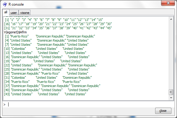
When executing this you see just the list of vertex names which are here the numbers from 1 to 45. To obtain the values of an attribute (e.g., Afrm) type
V(egonet)$Afrm
which returns the vector of countries of origin of the various actors.
Useful summary statistics include information about how many actors originate from the various countries. However, typing the command
summary(V(egonet)$Afrm)
just outputs information about the class and size of the list of countries of origin:
 Length   Class      Mode
 45       character  character
which is not very informative. To obtain the list of unique values for the Afrm attribute, you can type
unique(V(egonet)$Afrm)
which returns the names of five different countries. To count the number of actors in each of the countries, it is most convenient to convert the vector of character strings into a factor and save this factor in a new variable (e.g., called from) by typing the command
from <- as.factor(V(egonet)$Afrm)
Finally the command
summary(from)
returns the list of unique values along with the number of actors in each of the classes. In our example this is
 Colombia   Dominican Republic  Puerto Rico  Spain  United States
 2          14                  5            1      23
Indexing of vertex and edge iterators
Vertex iterators can be restricted to subsets by specifying a logical vector (or a command that produces one) in square brackets after the iterator. For instance, the command
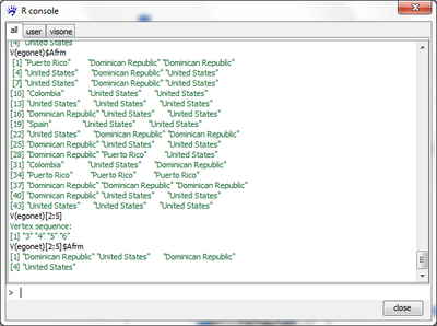
V(egonet)[2:5]
returns the values 3 to 6. This seeming contradiction is explained by the fact that counting of indices in vertex or edge iterators starts at zero; thus, the name of the vertex at position 0 is 1, the name of the vertex at position 2 is 3, and so on. The result of such a restriction operation on an vertex iterator is itself a vertex iterator and, thus, provides access to vertex attributes. For instance, typing
V(egonet)[2:5]$Afrm
returns the countries of origin of actors indexed by 2 to 5 (i.e., named 3 to 6). The command
V(egonet)[Acit == "new york"]$Afrm
gives you the countries of origin of all actors whose attribute Acit (encoding the city of residence) equals new york, and so on.
An edge iterator is returned via the command
E(egonet)
and offers access to edge attributes similar as for vertices.
Vertex iterators and edge iterators can be indexed by more complex conditions. Actually, any logical vector whose length equals the number of vertices (respectively edges) can be used as an argument in the square brackets following vertex iterators (respectively edge iterators). The following lines illustrate such indexing tasks. To select all actors whose origin is in the US and save this iterator in a variable actors.from.usa type
actors.from.usa <- V(egonet)[Afrm == "United States"]
All edges connecting two actors from the US are obtained by
edges.within.usa <- E(egonet)[actors.from.usa %--% actors.from.usa]
The command %--% is a special command used in edge iterators between two vertex iterators; it selects all edges connecting vertices from the two specified subsets (which might be identical, as in the example above). Edges with at least one actor from the US are selected by
edges.incident.usa <- E(egonet)[adj(actors.from.usa)]
To select all edges within any of the classes defined by Afrm we first construct a logical vector for edges that is true if and only if the Afrm attribute of the two connected vertices is identical and then use it as an argument in E(egonet)[...]. Therefore type
 el <- get.edgelist(egonet) +1
 within.class.edges <- V(egonet)[el[,1]]$Afrm == V(egonet)[el[,2]]$Afrm
 E(egonet)[within.class.edges]
The variable el is just a matrix with two columns containing the vertex ids of adjacent vertices. The +1 in the first line is necessary because ids start with zero.
Vertex and edge iterators can be restricted in various other ways; see the igraph documentation for details.
Analyzing distributions of centralities in igraph
The igraph package offers methods to compute various established centrality measures (refer to the igraph documentation for a complete list of available methods). While many of these could also be directly computed in visone without the detour via the R console, R directly offers statistical descriptions and analysis of the computed values. This is demonstrated in the following. The vertex degrees are returned by the command
degree(egonet)
Let's save this vector in a variable d by typing
d <- degree(egonet)
Mean, standard deviation, and summary statistics (including min, max, quartiles, and median) are computed by
 mean(d)
 sd(d)
 summary(d)
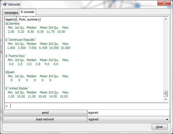
To display these (or other) statistics separately for each class of actors defined by the country of origin (or any other attribute), execute the command
tapply(d, from, summary)
The three arguments of tapply have the following meaning: d is the vector of values to which the function should be applied, from is the factor whose unique values determine the different classes, and summary is the function to be computed (instead of summary, you could also type mean, sd, and so on).
Loading networks from R into visone
As networks can be sent from visone to R, you can also load objects of class igraph into visone. Loading the current R object egonet would be of no use since this network is already in visone and has not been modified. Loading networks from R into visone is useful when some values that have been computed in R and attached to the igraph object should be accessible as vertex or edge attributes in visone. This offers numerous possibilities to transform attributes, as it will be demonstrated in the following.
First let's copy egonet into a new igraph object named g by executing
g <- egonet
(This rather serves to demonstrate how new variables for igraph objects can be loaded into visone; we could also have attached the new data directly to egonet.) To attach a new attribute named Degree that encodes the previously computed node degrees type
V(g)$Degree <- d
Degrees could have been computed in visone as well. However, R offers methods to transform such values that are not implemented directly in visone. For instance, the variable DegreeCentered computed and attached via
V(g)$DegreeCentered <- d-mean(d)
encodes the differences between the individual degrees and the mean (so that nodes with relatively small degrees get negative values and nodes with relatively high degrees get positive values). Likewise
V(g)$LogDegree <- log(d)
attaches the logarithmized degrees to the graph (this transformation is quite useful in networks with skewed degree distributions, e.g., preferential attachment graphs). Note that while visone directly offers some possibilities to transform attributes, logarithmic transformations are not implemented; in contrast, R as a programming language, imposes no such restrictions.
Finally, loading the network along with all old and new attributes into visone can be done via the R console tab as explained in the following. Click once on the refresh button to show all R variables of class igraph (note that this shows the variable g but not the vector of degrees d). Selecting g and pushing the load button opens a new network tab with a network called g. You can inspect the newly attached attributes via the attribute manager.
File import and export in R
Saving and loading R objects
Variables in the R workspace can be saved to and read from the disk. If you just want to save the igraph objects (the network together with all attributes) you could as well load them into visone and save them as GraphML. However, your R workspace might contain other variables that are not of class igraph. To save objects it is convenient to set the working directory. The path to the current working directory can be obtained by
getwd()
which currently outputs in many cases the directory where the Rserve.exe file is located (see the R connection settings). To set it to a different directory type
setwd("<path_to_directory>")
(Chose a directory to which you have write-access.) Saving an R object (for instance, the network egonet) can be done by
save(egonet, file="egonet.rda")
This creates a file egonet.rda in the specified working directory. (Here, egonet.rda is an arbitray filename that you can chose as you wish. ) All objects in the workspace can be saved by
save.image(file="myWorkspace.rda")
Conversely, to read objects from a file in the current working directory type
load(file="egonet.rda")
(This makes sense if you have closed the R connection and you want to recover the object egonet.) R objects that have been saved to disk can, of course, also been imported into any other R environment (see http://www.r-project.org/ for more information).
Plotting to a PDF file
To plot a diagram, such as the degrees of a network, to a PDF file type
 pdf("myDiagram.pdf")
 plot(d, type="b")
 dev.off()
This writes a PDF file myDiagram.pdf to the current working directory; this file can be viewed, e.g., with Adobe's Acrobat Reader, printed, or used as a figure in some other document. The R plot command is a very general and powerful tool to create statistical graphics; for more information see the documentation linked from the R Project Website.
Executing R code from a file
Especially if you are working on a larger project it is convenient not just to save the data but also the R code to recompute some of the results or to modify some analyses. R code can be executed from text-files by the source command. For instance,
source("myRCode.R")
executes all commands from the file myRCode.R located in the current working directory. Note that this file must be a plain text file (see http://en.wikipedia.org/wiki/Text_editor for explanation) containing commands like the examples provided in typewriter font in the boxes on this page. Conversely,
sink("myROutput.txt")
directs the R output to a file myROutput.txt in the current working directory. This is convenient when executing R commands that produce complex output.
Fitting exponential random graph models (ERGMs)
Since networks can be sent from visone to R you get the possibility to use many powerful contributed R packages for network analysis and modeling. In this section we illustrate the use of some methods provided by the statnet package written by Mark S. Handcock, David R. Hunter, Carter T. Butts, Steven M. Goodreau, and Martina Morris; see the statnet project Website for additional information, including documentation and tutorials. In particular, we are going to demonstrate how to fit an exponential random graph model (ERGM) to a network sent from visone to R. ERGMs are sophisticated statistical network models that can deal with complex dependencies among observations, including homophily, reciprocity, preferential attachment, and triangular closure. Note that ERGMs are mainly applied to time-independent networks; an option for modeling network dynamics is the RSiena package that can be used from within visone as it is illustrated in the RSiena tutorial.
Installing new packages
To estimate an ERGM we need to install the R packages network, sna, and ergm, all of which are part of the statnet package. To install these packages separately type (after appropriate replacement of <path to R library dir> and <url of R mirror site>)
 install.packages("network", lib = "<path to R library dir>", repos = "<url of R mirror site>")
 library(network, lib.loc = "<path to R library dir>")
 install.packages("sna", lib = "<path to R library dir>", repos = "<url of R mirror site>")
 library(sna, lib.loc = "<path to R library dir>")
 install.packages("ergm", lib = "<path to R library dir>", repos = "<url of R mirror site>")
 library(ergm, lib.loc = "<path to R library dir>")
For the R library you can set the same path as in the R connection settings; a list of mirror sites can be found at http://cran.r-project.org/mirrors.html (copy the URL of any mirror site, including the http:// prefix, and use it in quotes as a value for the repos argument in the commands above).
Since igraph and network are both packages for networks, they define some methods with identical names. This can lead to problems when a method from one package is executed on an object from the other. A workaround for such problems would be to save the objects that you want to work with, close the R connection, open it again, install only the package that you need, and reload the data objects.
Converting an igraph to a network object
The ergm package works on network objects from the package network. Thus, the current igraph object first has to be converted into this class. This can be done in two steps: getting the adjacency matrix for the egonet object by
adj <- get.adjacency(egonet)
and then creating a network from this adjacency matrix by executing the following line (note that the directed attribute must be set to FALSE, otherwise the network will be directed)
net <- as.network(adj, directed=FALSE)
Executing
summary(net)
shows that the ties have been correctly converted from the igraph package to network but, so far, no vertex or edge attributes are attached to the net object. This can be done by, e.g.,
 set.vertex.attribute(net,"From", V(egonet)$Afrm)
 set.vertex.attribute(net,"City", V(egonet)$Acit)
Conversely, to create an igraph from an adjacency matrix use the command graph.adjacency(adj, mode="undirected") (we don't need this at the moment).
Computing observed statistics
The ergm package enables the computation of the observed values of various network statistics, such as number of triangles, number of k-stars, and many more. To get these values call the summary method on an ERGM formula object. For instance,
summary(net ~ triangle + kstar(2) + nodematch("City"))
returns the number of triangles in the network, the number of 2-stars, and the number of edges connecting actors that live in the same city. In our example, this is
 triangle   kstar2   nodematch.City
 543        1857     143
To see other statistics that can be used in an ERGM formula see the section on ergm.terms in the statnet documentation linked from http://statnetproject.org.
Estimating ERGMs
Exponential random graph models (ERGMs) assign a network a probability of the form
, where
- the are functions mapping from the set of networks (the population of the random graph model) to the real numbers; the are called (network) statistics and are typically chosen by the researcher based on theory
- is a vector of free parameters associated with statistics; the parameters are typically estimated via maximum likelihood estimation (MLE) given an observed network
- is a normalization constant for the random graph model
The statistics are typically (functions of) counts of small subgraphs such as edges, stars, triangles, or edges connecting actors that have specific attribute values. The interpretation of the estimated parameters is as follwing. If, for instance, the parameter associated with the triangle count statistic is (significantly) positive, then networks with more triangles have higher probability - assuming that all other statistics remain constant. This would demonstrate a tendency for transitive closure as described in the saying the friend of a friend is a friend. The specification, estimation, and interpretation of ERGMs is quite involved and cannot be sufficiently treated in this page; for more information we refer to the statnet tutorial linked from http://statnetproject.org. In the following, we illustrate merely how ERGMs can be specified and estimated in statnet.
Computing maximum likelihood estimates for ERGM parameters can be done by calling the ergm on an ERGM formula. For instance,
model <- ergm(net ~ edges + nodematch("From") + nodematch("City") + gwesp(0.1, fixed=TRUE))
estimates the parameters of a model with four statistics: number of edges, numbers of edges connecting actors with the same country of origin, respectively the same city of residence, and the so-called geometrically weighted edgewise shared partners statistic. The latter has a similar interpretation as the triangle statistic but is less likely to lead to degenerate models; see the statnet documentation for details. Calling
summary(model)
prints basic information about the model, including estimated parameters and standard errors. In our example, we get (note that the results might change from call to call, since the estimation algorithm itself is probabilistic)
 ==========================
 Summary of model fit
 ==========================
 Formula:   net ~ edges + nodematch("From") + nodematch("City") + gwesp(0.1, fixed = TRUE)
 Newton-Raphson iterations:  6
 MCMC sample of size 10000
 Monte Carlo MLE Results:
                 Estimate     Std. Error MCMC s.e. p-value
 edges            -4.1438     3.8443     0.193     0.281
 nodematch.From    0.8223     0.1459     0.006     <1e-04 ***
 nodematch.City    0.8212     0.1553     0.002     <1e-04 ***
 gwesp.fixed.0.1   3.0107     3.4763     0.175      0.387
 ---
 Signif. codes:  0 '***' 0.001 '**' 0.01 '*' 0.05 '.' 0.1 ' ' 1
    Null  Deviance: 1372.43  on 990  degrees of freedom
 Residual Deviance:  484.89  on 986  degrees of freedom
          Deviance:  887.54  on   4  degrees of freedom
 AIC: 492.89    BIC: 512.48
From these results we can conclude that ties are more likely between actors that stem from the same countries of origin (significantly positive estimate for the parameter associated with the nodematch.From statistic) and ties are more likely between actors that live in the same city (nodematch.City). We could not find evidence for transitive closure - controlling for country of origin and city of residence - since the parameter associated with gwesp.fixed.0.1 is not significant.
References
Gábor Csárdi and Tamás Nepusz. The igraph library. http://igraph.sourceforge.net/.
Mark S. Handcock, David R. Hunter, Carter T. Butts, Steven M. Goodreau, and Martina Morris (2003). statnet: Software tools for the Statistical Modeling of Network Data. URL http://statnetproject.org.
The R project for statistical computing http://www.r-project.org/
